5 Excel Find and Replace Tricks That Save Hours

Hi ,

Most Excel users know Find and Replace as the tool you use when you need to change one word, number, or label into something else.

But that is only the beginning.

Hidden behind the Options button in the Find and Replace dialog box are some incredibly useful features that can save hours of manual editing. You can use Find and Replace to change formatting without changing values, clean messy exported data, update formulas, replace values across an entire workbook, and even remove invisible line breaks from cells.

In this tutorial, you'll learn five powerful Excel Find and Replace tricks that go well beyond basic text replacement.

How to Open Find and Replace in Excel

The fastest way to open Find and Replace in Excel is with the keyboard shortcut:

Ctrl+H

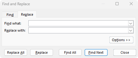
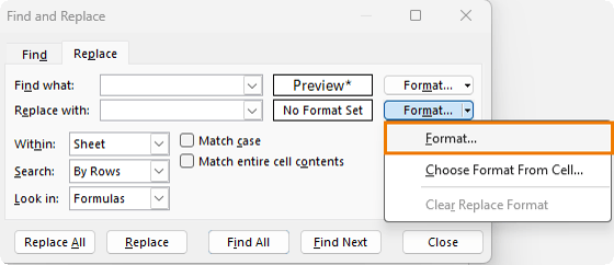
This opens the Replace tab of the Find and Replace dialog box:

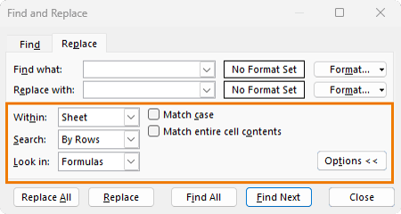
From there, click Options to reveal the advanced settings:

This is where you'll find many of the features that most Excel users overlook, including:

These options are what make Find and Replace far more powerful than most people realise.

1. Replace Cell Formatting Without Changing the Values

One of the most useful hidden features in Excel Find and Replace is the ability to find and replace formatting.

This is especially helpful when you need to update a report where certain cells are formatted in a specific way, but those cells are not all together in one range.

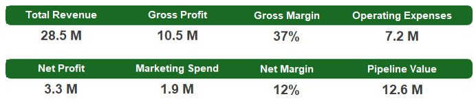
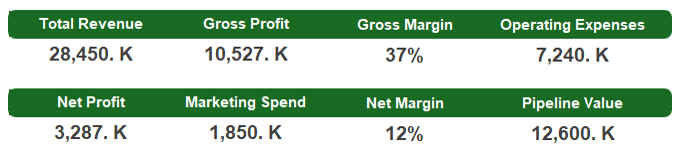
For example, imagine you have a report where large numbers are formatted in millions, like this:

Then your boss changes their mind and wants the same figures shown in thousands instead.

You could manually select every section of the report and change the number format one area at a time, but that is slow and easy to get wrong, especially when the cells are scattered throughout the worksheet.

Instead, you can use Find and Replace to find cells with the current number format and replace that format with a new one.

How to Replace Number Formatting in Excel

1. Press Ctrl+H to open Find and Replace.

2. Click Options.

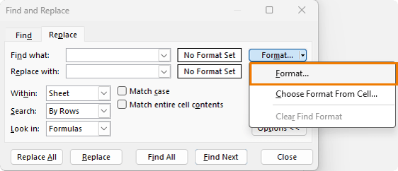
3. Next to Find what, click the Format dropdown:

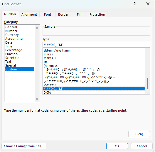
4. Choose the existing format you want Excel to find:

5. Next to Replace with, click Format:

6. Choose the new number format.

7. Click Replace All.

For example, if the current format is:

#,##0.0,, "M"

You could replace it with:

#,##0, "K"

This changes the display from millions to thousands without changing the underlying numbers:

That distinction is important. The values in the cells remain untouched. Only the way those values are displayed changes.

Important Tip: Clear the Find Format Afterwards

Excel remembers the last format you searched for.

This can cause confusion the next time you use Find and Replace because Excel may still be looking for that previous format in the background.

After using Find and Replace with formatting:

1. Open Find and Replace again with Ctrl+H.

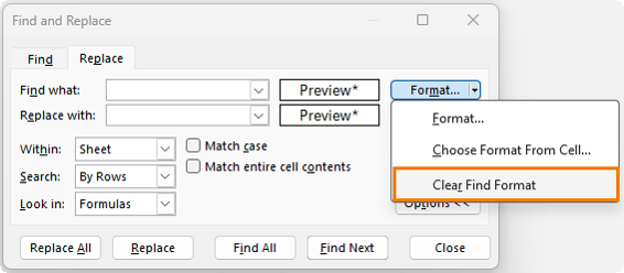
2. Click the dropdown arrow next to Format.

3. Choose Clear Find Format.

This resets the search criteria and helps avoid those frustrating moments where Find and Replace appears not to work.

2. Use Wildcards in Excel Find and Replace

Wildcards are not just for formulas. They also work inside Excel Find and Replace.

This is incredibly useful when cleaning messy data from bank exports, accounting systems, CRMs, ecommerce platforms, or other external sources.

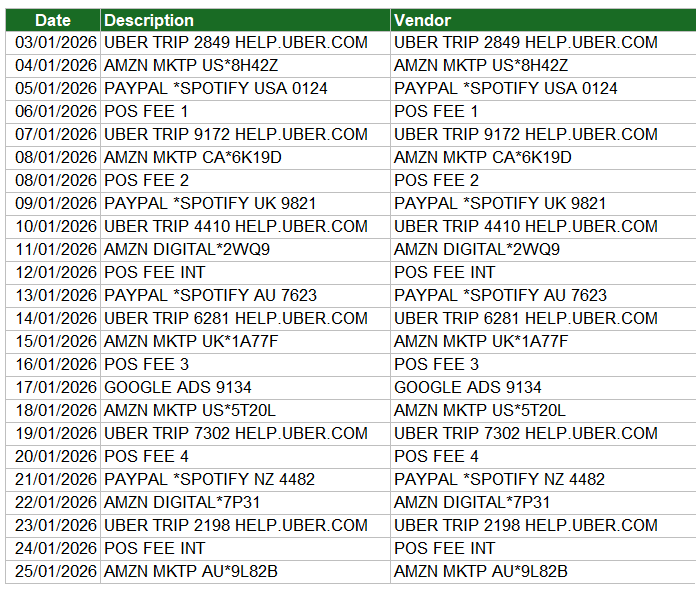
For example, bank transaction descriptions often contain extra details such as:

A transaction might look like this:

UBER TRIP 2849 HELP.UBER.COM

But for reporting, you may only want the clean vendor name:

Uber

This is where wildcards help.

What Does the Asterisk Wildcard Do in Excel Find and Replace?

The asterisk wildcard, *, means:

Match any number of characters.

So if you search for:

UBER*

Excel finds anything that starts with UBER, regardless of what comes after it.

You can then replace all those messy descriptions with:

Uber

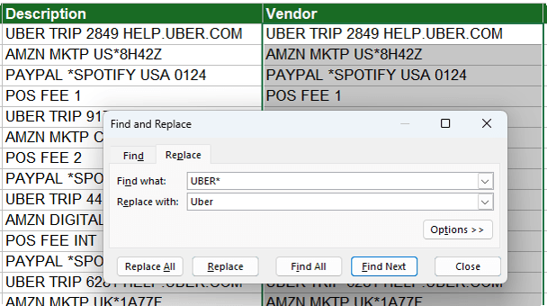
Example: Clean Uber Transactions in the Vendor column:

1. Press Ctrl+H.

2. In Find what, enter: UBER*

3. In Replace with, enter: Uber

4. Click Replace All.

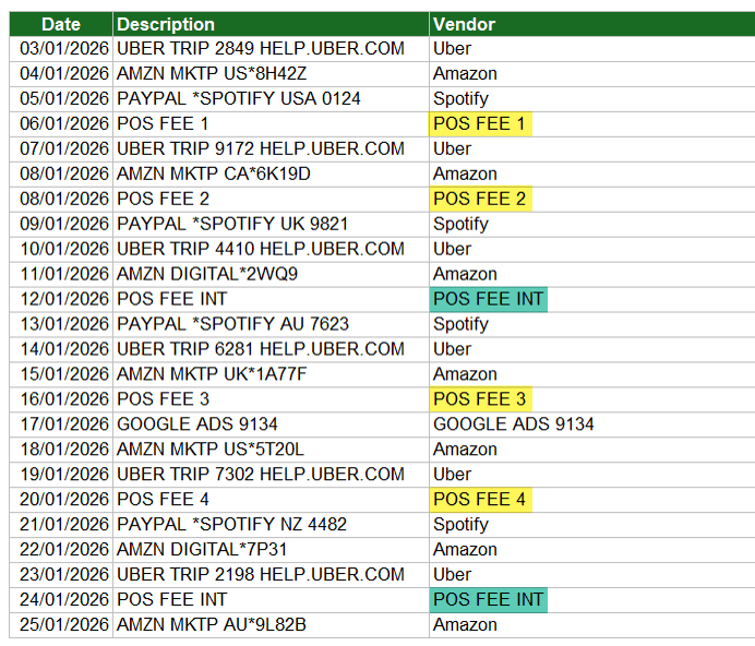
Excel replaces all descriptions that start with UBER with the clean vendor name.

Clean Amazon Transactions with Wildcards

You can use the same technique for Amazon transactions.

A bank export might contain descriptions like:

AMZN MKTP US*8H42Z

The marketplace code changes each time, but the transaction usually starts with AMZN.

Search for:

AMZN*

Replace with:

Amazon

This turns inconsistent Amazon transaction descriptions into one clean vendor name.

Find Text Anywhere in a Cell with Wildcards

Sometimes the text you want to find does not appear at the start of the cell.

For example, a Spotify payment might look like this:

PAYPAL *SPOTIFY USA 0124

In this case, Spotify appears somewhere in the middle of the text string.

To find anything containing Spotify, search for:

*SPOTIFY*

Replace with:

Spotify

This tells Excel to find any cell that contains Spotify anywhere in the text.

What Does the Question Mark Wildcard Do in Excel Find and Replace?

The question mark wildcard, ?, is more precise than the asterisk.

It means:

Match exactly one character.

This is useful when you want to replace values that follow a very specific pattern.

For example, you might have bank fees like:

POS FEE 1
POS FEE 2
POS FEE 3
POS FEE 4

But you may also have:

POS FEE INT

If you want to replace the single-digit fee codes without changing POS FEE INT, you can use the question mark wildcard.

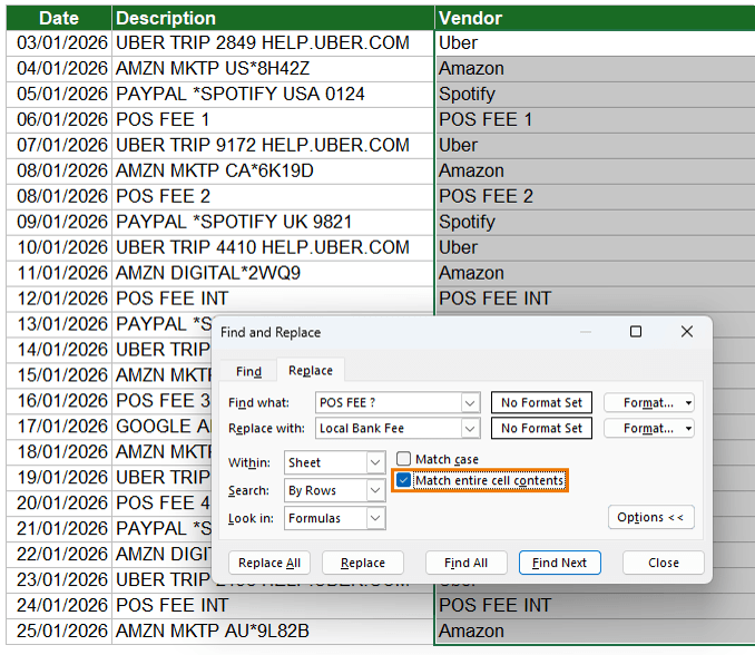
Search for:

POS FEE ?

Replace with:

Local Bank Fee

The question mark matches one character only, so it can match POS FEE 1, POS FEE 2, and POS FEE 3.

However, there is one more setting to use here.

Use Match entire cell contents for safer replacements.

When using precise wildcard patterns, turn on Match entire cell contents.

This ensures Excel only replaces cells where the whole cell matches the pattern.

Without this option, Excel may find and replace part of a longer text string, which could lead to unwanted changes.

To use it:

1. Press Ctrl+H.

2. Click Options.

3. Enter your wildcard search.

4. Tick Match entire cell contents.

5. Click Replace All.

The key difference is:

The asterisk is broad. The question mark is specific.

Use the asterisk when the text length varies. Use the question mark when you need to match a fixed number of characters.

3. Replace Text Inside Formulas, Not Values

Find and Replace can search the values displayed in cells, but it can also search the formulas behind those cells.

This is one of the most useful settings when you need to fix formulas across a worksheet or workbook.

A common example is when you copy a worksheet from one workbook to another.

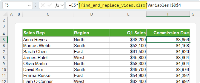
If the formulas in the copied sheet referenced other sheets in the original workbook, Excel may prefix those references with the original file name.

For example, a formula might contain a reference like:

[find_and_replace_video.xlsx]

Usually, this is not what you want.

You might be able to fix one formula manually, but if there are formulas scattered throughout the worksheet, manually editing each one can be risky and time-consuming.

Find and Replace can fix them all at once.

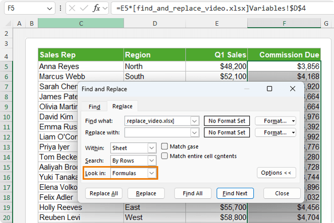
How to Use Find and Replace in Excel Formulas

1. Click into a formula that contains the unwanted workbook reference.

2. Copy the file path or workbook reference you want to remove.

3. Press Ctrl+H.

4. Paste the unwanted reference into Find what.

5. Leave Replace with blank, or enter the replacement text if needed.

6. Click Options.

7. Set Look in to Formulas.

8. Click Replace All.

Excel updates the formulas themselves, not just the displayed values.

This is especially useful for:

The important setting is Look in: Formulas.

If you leave this set to Values, Excel may not find what you need because it is only looking at the result displayed in the cell, not the formula behind it.

4. Replace Across an Entire Workbook

By default, Excel Find and Replace searches only the active sheet.

But you can change that.

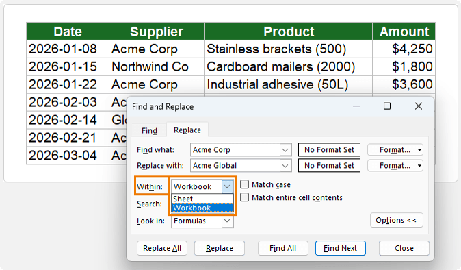
Inside the advanced options, there is a Within dropdown. This lets you choose whether to search within the current sheet or the entire workbook.

This is ideal when you need to update the same text across multiple worksheets.

For example, imagine you have three regional sales sheets:

Each sheet contains a supplier name:

Acme Corp

The supplier has rebranded and now needs to be shown as:

Acme Global

Instead of updating each worksheet separately, you can replace the name across the whole workbook in one step.

How to Find and Replace Across a Workbook in Excel

1. Press Ctrl+H.

2. Click Options.

3. Change Within from Sheet to Workbook.

4. In Find what, enter: Acme Corp

5. In Replace with, enter: Acme Global

6. Click Find All first.

7. Review the results.

8. If everything looks correct, click Replace All.

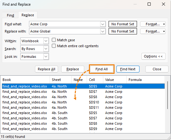
Why You Should Use Find All Before Replace All

When replacing across an entire workbook, it is safer to click Find All before clicking Replace All.

Excel will show a list of every match it found, including the sheet name, cell address, and value:

This gives you a chance to check the results before committing to the replacement.

If something does go wrong, you can usually press Ctrl+Z to undo the whole batch in one step. However, it is always better to check first, especially when working with large files or important reports.

5. Replace Line Breaks in Excel Cells

One of the least obvious Find and Replace tricks in Excel is replacing line breaks.

This is useful when data has been copied from an email, PDF, web page, or system export and each item appears on multiple lines inside the same cell.

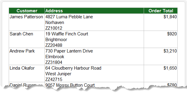
For example, you may have addresses where the street, city, and postcode are separated by line breaks inside one cell:

That might look fine visually, but it can cause problems when you want to:

To clean it up, you can replace the line breaks with a comma and space.

The Hidden Character Behind Excel Line Breaks

A line break inside a cell is created by a hidden character.

In formulas, you may know this as:

=CHAR(10)

However, you cannot type CHAR(10) into the Find and Replace dialog box as a formula.

Instead, you need to enter the line break character directly using a keyboard shortcut.

That shortcut is:

Ctrl+J

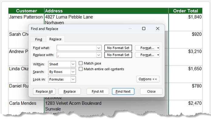
How to Replace Line Breaks in Excel

1. Select the cells containing line breaks.

2. Press Ctrl+H.

3. Click inside the Find what box.

4. Press Ctrl+J.

The Find box will look empty. That is normal. The line break character is invisible.

5. In Replace with, type a comma and a space: ', '

NOTE: The single quotes are just to show the space after the comma

6. Click Replace All.

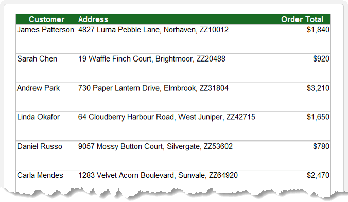
Excel removes the line breaks and replaces them with commas, putting the text onto one line:

Now, an address stored over three lines inside one cell is a single clean address separated by commas.

Important Tip: Clear Ctrl+J After Replacing Line Breaks

Excel can remember the invisible Ctrl+J character the next time you use Find and Replace.

This can make your next search behave strangely because the Find box may look empty even though it still contains the hidden line break character.

To clear it:

This removes the invisible character so you can start a normal Find and Replace again.

Final Thoughts

Find and Replace is one of those Excel tools most people think they already know.

But once you open the advanced options, you'll find features that can save huge amounts of time, especially when cleaning data, updating reports, fixing formulas, or making changes across a workbook.

The next time you reach for Find and Replace, don't just type the text and click Replace All. Open Options first.

That is where Excel hides the features that make this tool genuinely powerful.

Have a great day,

Mynda Treacy

Co-founder My Online Training Hub