Formula-Driven Summaries Without PivotTables
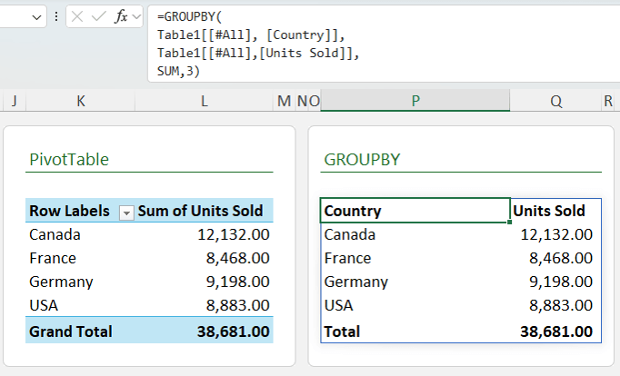
The GROUPBY function allows you to group and summarise data using a single formula.
Conceptually, it works like a PivotTable, but instead of a static object, you get a fully dynamic formula result that updates instantly when your data changes.
GROUPBY Syntax:
=GROUPBY(group_by, values, function, [header], [totals], [sort_order], [filter])
With GROUPBY, you specify:
- The column or columns you want to group by
- The values you want to aggregate
- The aggregation function such as SUM, AVERAGE, COUNT, or a custom LAMBDA
- Whether headers and subtotals should be included
Because GROUPBY outputs a spilled array, you can feed its results directly into other formulas, apply conditional formatting, or connect it to slicers. This makes it ideal for building flexible reports without the overhead of PivotTables.
The example below, shows the PivotTable on the left recreated with the GROUPBY function on the right:
GROUPBY also supports grouping by multiple columns, sorting results, filtering rows before aggregation, and controlling subtotal behaviour, all from within the formula itself.
💡Check out the deep dive GROUPBY function tutorial for more.
PivotTable Layouts With a Single Formula
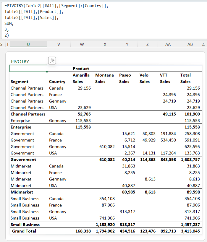
The PIVOTBY function takes the idea of GROUPBY one step further by allowing you to pivot results across columns as well as rows.
PIVOTBY
Syntax:
=PIVOTBY(row_fields, column_fields, values, function, [header], [totals], [sort_order], [filter])
With PIVOTBY, you define:
- One or more row grouping fields
- A
column field to pivot across
- The values to summarise
- The aggregation function
- Header, subtotal, and grand total behaviour
The result is a PivotTable-style layout created
entirely with a formula. This means it updates automatically, can be referenced by other formulas, and avoids the refresh and layout limitations of traditional PivotTables.
The PIVOTBY formula below displays data summarised by segment and country down the rows and product across the columns:
Like GROUPBY, PIVOTBY also supports sorting, filtering, and custom calculations, making it ideal for modern dashboards and
dynamic reports.
With a clever technique, GROUPBY and PIVOTBY outputs can even be connected to slicers, allowing interactive filtering without PivotTables.
💡Check out the deep dive PIVOTBY function tutorial for more.
Excel’s Modern Array Shaping Toolbox
Modern Excel includes a powerful set of lightweight array shaping functions that let you reshape, trim, and
reorganise data in seconds. These functions replace many older techniques involving OFFSET, helper columns, or complex nested formulas.
Dynamic Ranges Made Easy
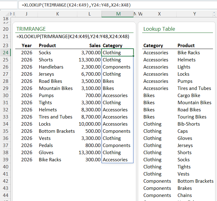
The TRIMRANGE
function simplifies dynamic ranges by removing trailing or leading empty rows and columns. This means formulas no longer waste resources calculating empty cells.
TRIMRANGE Syntax:
=TRIMRANGE(range, [row_trim_mode],
[col_trim_mode])
Instead of using volatile functions like OFFSET, you can use TRIMRANGE to create clean, efficient, dynamic references that automatically expand as data grows.
TRIMRANGE Example:
In the image below TRIMRANGE references to cell K49, but because there is no data in rows 40:49, it only returns results to row 39:
Even better, Excel introduces a shorthand dot operator that allows you to trim ranges directly inside formulas. By placing a dot after the colon, Excel trims trailing blanks automatically. By placing dots on both sides, you can trim both leading and trailing blanks.
The example below shows how we can simplify the formula above using TRIMRANGE with the dot operators:
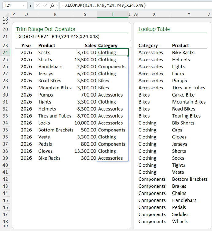
This is especially powerful when working with dynamic array formulas like XLOOKUP, SCAN, and FILTER, and it solves a common limitation where spilled formulas cannot be placed inside Excel Tables.
For large datasets, TRIMRANGE and the dot operator can significantly improve performance and clarity.
💡Check out the deep dive TRIMRANGE function tutorial for more.
Flatten Data Instantly
TOCOL reshapes any range
into a single column, while TOROW reshapes data into a single row.
TOCOL Syntax:
=TOCOL(array, [ignore], [scan_by_column])
TOROW
Syntax:
=TOROW(array, [ignore], [scan_by_column])
These functions allow you to:
- Ignore blank cells
- Control whether Excel scans by row or by column
- Prepare data for validation lists, analysis, or downstream formulas
They are especially useful when working with data that arrives in inconsistent layouts or needs to be normalised quickly.
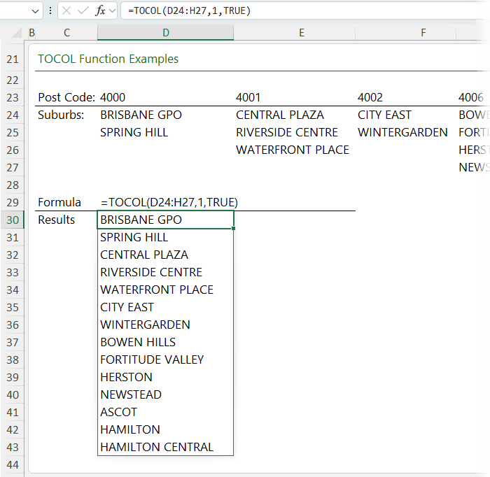
The TOCOL example below
rearranges the data in cells D24:H27 into a vertical list:
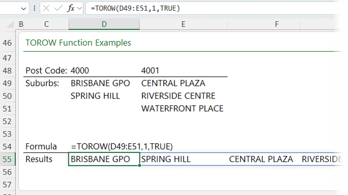
And the TOROW example below rearranges columns D and E of data into a horizontal list:
Extract Exactly What You
Need
CHOOSECOLS returns only the columns you specify from a range or array. CHOOSEROWS does the same for rows.
CHOOSECOLS Syntax:
=CHOOSECOLS(array, col_num1, [col_num2], …)
CHOOSEROWS Syntax:
=CHOOSEROWS(array, row_num1, [row_num2], …)
Both functions support positive and negative indexing, which means you can easily extract the first, last, or specific
positions without counting columns manually.
These functions make it simple to reorder data, isolate key fields, or pass only relevant portions of an array into another formula.
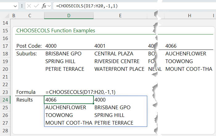
Take the CHOOSECOLS example below that extracts the last and first columns in that order:
💡Check out the video above for more examples, including for CHOOSEROWS.
Precise Control Over Array Output
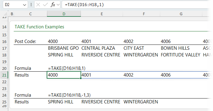
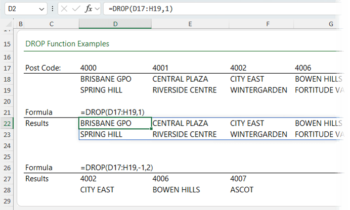
TAKE keeps a specified number of rows or columns from the beginning or end of an array. DROP removes rows or columns instead.
TAKE Syntax:
=TAKE(array, rows, [columns])
DROP Syntax:
=DROP(array,
rows, [columns])
They are perfect for:
- Removing headers or footers
- Keeping only recent records
- Preparing clean inputs for other functions
Together, TAKE and DROP provide fine-grained control over dynamic array outputs with minimal syntax.
The TAKE examples below show the use of both positive and negative values in the rows and columns arguments:
Likewise for DROP:
Reshape Lists Visually
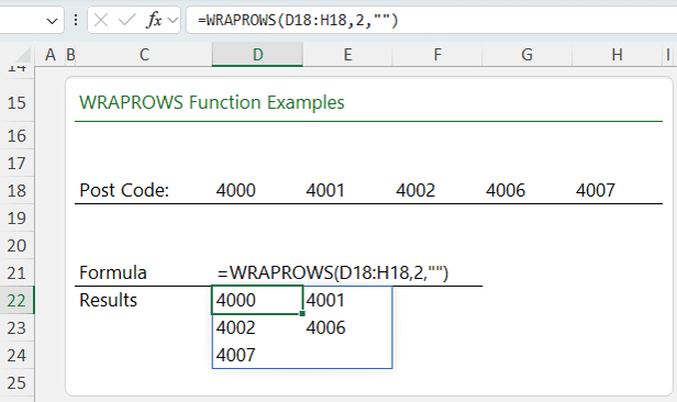
WRAPROWS reshapes a single list into multiple rows, while WRAPCOLS reshapes data into multiple columns.
WRAPROWS Syntax:
=WRAPROWS(array, wrap_count, [pad_with])
WRAPCOLS Syntax:
=WRAPCOLS(array, wrap_count,
[pad_with])
You control:
- How many values appear per row or column
- What appears in padded cells when the data does not fit evenly
These functions are ideal for formatting
outputs, building printable layouts, or reshaping lists for presentation, like the list of post codes below wrapped into rows across multiple columns:
Enforce a Consistent Array Shape
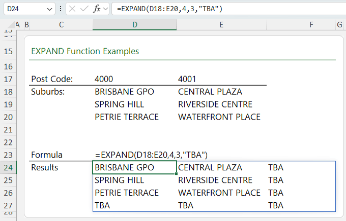
EXPAND increases an array to a fixed number of rows or columns and pads missing values with a specified placeholder.
EXPAND Syntax:
=EXPAND(array, rows,
[columns], [pad_with])
This is particularly useful when:
- Passing arrays into other functions that expect a consistent shape
- Building templates where outputs must align perfectly
- Avoiding spill errors caused by
mismatched dimensions
The EXPAND formula below pads the original array with an additional row and column:
Dynamic Running Totals and Beyond
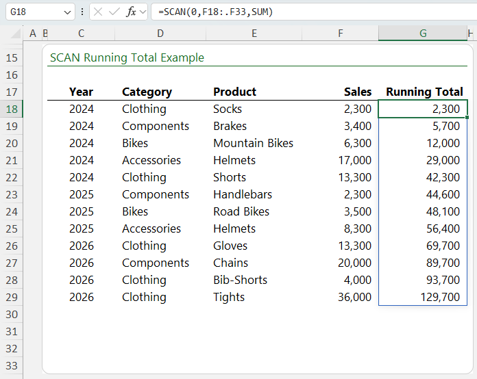
SCAN calculates cumulative results across an array and returns every intermediate value, not just the final total.
SCAN Syntax:
=SCAN(initial_value, array, LAMBDA(accumulator, value))
While the syntax may sound complex, SCAN is extremely intuitive for tasks like:
- Running totals
- Rolling calculations
- Trend analysis
- Helper arrays for advanced formulas
Because SCAN works with dynamic ranges and supports the trim reference dot operator (shown below), it automatically expands as new data is added.
Insert Images Directly Into Cells
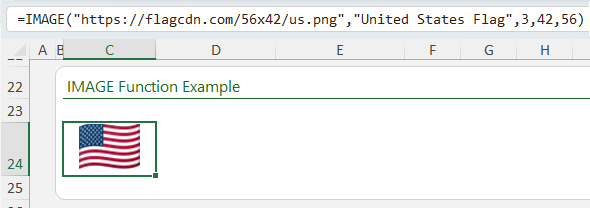
The IMAGE function allows you to insert images into cells using a formula.
IMAGE Syntax:
=IMAGE(source, [alt_text], [sizing], [height], [width])
You can:
- Reference images via URLs
- Add alternative text for accessibility
- Control sizing behaviour
- Specify exact height and width
Because images live inside cells, they respect alignment, sorting, filtering, and layout rules
just like text. This makes IMAGE ideal for dashboards, product lists, icons, and visual indicators.
💡Check out the deep dive IMAGE function tutorial for more.
AI Inside Excel Formulas
The
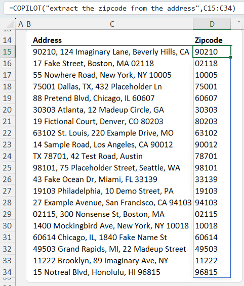
COPILOT function brings generative AI directly into Excel formulas. It’s available with Microsoft 365 and a Copilot license.
COPILOT Syntax:
=COPILOT(prompt, [input], [parameters])
Instead of calculating numbers, COPILOT interprets prompts and data to:
- Extract unstructured information
- Reformat inconsistent text
- Classify or summarise data
- Generate explanations or examples
It excels at tasks that are difficult or impossible with traditional formulas, such as parsing messy
addresses or rewriting text into a standard format.
COPILOT is designed for exploratory and generative tasks, not numeric calculations, and it represents a fundamental shift in how Excel can be used.
In the example below it easily extracts the zip code from the unstructured address
data:
What Comes Next
The COPILOT function is only the beginning. Excel’s Copilot Agent Mode takes automation even further by planning workflows, reading entire workbooks, building multiple sheets, writing formulas, creating dashboards, and documenting every decision from a single prompt.
If you are excited about the future of Excel and want to combine AI with your own expertise, learning how to use Copilot Agent Mode
effectively is the next step.
Want to Master These Skills Faster?
If you are reading this and thinking you want to write these formulas confidently and understand how they fit together, the Advanced Excel Formulas course is the perfect next step.
It takes you from long, messy formulas to clean, flexible solutions using dynamic arrays, LET, LAMBDA, and the modern functions analysts rely on today.