1. Lookup Functions – Connect & Reshape Data
XLOOKUP
The modern replacement for VLOOKUP and HLOOKUP, XLOOKUP is the one lookup function you’ll ever need. It allows you to search for values in a table or range and return corresponding results across multiple columns.
XLOOKUP Syntax: XLOOKUP(lookup_value, lookup_array, return_array, [if_not_found], [match_mode], [search_mode])
Example data:
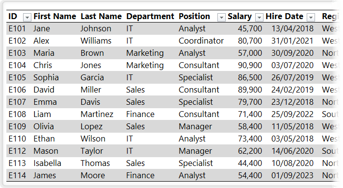
Let’s say we want to lookup
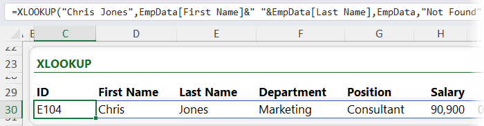
Chris Jones’ data in the table above named ‘EmpData’ using XLOOKUP. We can write it like this:
=XLOOKUP(“Chris Jones”, EmpData[First Name]&" "&EmpData[Last Name], EmpData, "Not Found")
Note: in the lookup_array argument above I’ve had to concatenate the First Name and Last Name columns together because we’re looking up the full name. However, if you have a lot of XLOOKUP formulas, it would be more efficient to add a column to the employee table that joins the first and last names together and reference that in the
lookup_array, rather than referencing the two separate columns in the formula.
In the image below you can see the results of the XLOOKUP formula spill across the columns:
🎓Get up to speed with the XLOOKUP function
here.
FILTER
The FILTER function extracts only the rows you need
based on conditions. It’s perfect for dynamic reporting.
FILTER Syntax:
FILTER(array, include, [if_empty])
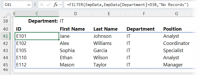
Using the same example
data, let’s say I want to extract a list of the IT department employees. I can write the FILTER formula like this:
=FILTER(EmpData, EmpData[Department]=D39, "No Records")
In the image below we can see the result:
🎓Get up to speed with the FILTER function here.
SORT + UNIQUE
Combine the UNIQUE function to generate distinct lists and the SORT function to arrange them in ascending or descending order. Ideal for creating dropdown menus or data validation lists.
UNIQUE Syntax: UNIQUE(array, [by_col], [exactly_once])
SORT
Syntax: SORT(array, [sort_index], [sort_order], [by_col])
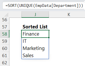
We can write the formula to extract a sorted unique list of department names like this:
=SORT(UNIQUE(EmpData[Department]))
🎓Get up to speed with the UNIQUE function here and the SORT function here.
2. Logic Functions – Test, Decide, Control
IF, OR, AND
The IF function checks
conditions and returns different results depending on whether the condition is TRUE or FALSE. Combined with OR and AND, you can build powerful logical tests.
IF syntax:
IF(logical_test,[value_if_true],[value_if_false])
OR syntax:
OR(logical1,logical2,...)
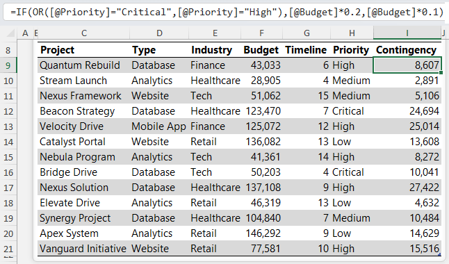
Example – let’s say we want to add a 20% budget contingency
for projects that are Critical OR High priority, with all other projects receiving a 10% contingency. We would write the formula like this:
=IF(OR([@Priority]="Critical",[@Priority]="High"),[@Budget]*0.2,[@Budget]*0.1)
And you can see the results in column I of the image
below:
🎓Get up to speed with IF, AND, OR functions here.
Nested IF & IFS
For multiple conditions, you can nest IF statements or use the IFS
function. Nested IFs stop evaluating once a condition is TRUE, making them more efficient in many cases.
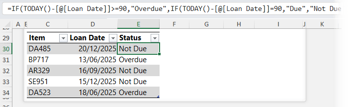
For example, let’s say I want to identify which of the items below are Due, Overdue or Not Due. The loan period is 90 days. I could write a nested IF formula like this:
=IF(TODAY()-[@[Loan Date]]>=90,"Overdue",IF(TODAY()-[@[Loan Date]]=90,"Due","Not Due"))
And the image below you can see the result in column E:
3. Conditional Aggregations – Summarise Data with Criteria
SUMIFS
Adds values based on
multiple conditions.
SUMIFS Syntax:
SUMIFS(sum_range, criteria_range, criteria,...)
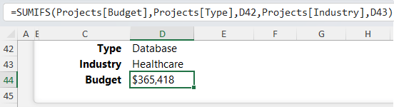
For example, using the data from the IF function example let’s say I want to sum the budgets for Database projects in the
Healthcare industry. We can do so with this formula:
=SUMIFS(Projects[Budget], Projects[Type], D42, Projects[Industry], D43)
In the screenshot below you can see cell D42 contains the Type and D43 contains the Industry:
Tip: you can keep adding criteria range and criteria pairs as
required.
🎓Get up to speed with SUMIFS here.
COUNTIFS
Counts rows that meet specific criteria. It has a slightly simpler syntax than SUMIFS because we only need to specify criteria.
COUNTIFS syntax:
COUNTIFS(criteria_range,criteria,...)
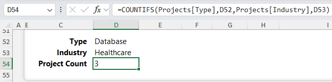
For example, we can count the project types for Database and where the industry is Healthcare with this formula:
=COUNTIFS(Projects[Type], D52, Projects[Industry], D53)
In the screenshot below you can see cells D52 contains the Type and D53 contains the
Industry:
Tip: for homework try out the AVERAGEIFS, MINIFS, MAXIFS functions, which are all variations of SUMIFS.
🎓Get up to speed with COUNTIFS here.
4. Date Intelligence Functions – Aggregate, Forecast, Schedule
EOMONTH
Finds the first or last date of a month - vital for monthly reporting.
EOMONTH
syntax:
EOMONTH(start_date, months)
For example, let’s say the current date is 7th October 2025 and from this date we need to derive the end of the month. We can use EOMONTH like so:
=EOMONTH(DATE(2025,10,7),0)
Which returns October 31, 2025.
We can also use EOMONTH as criteria arguments for SUMIFS.
For example, here I have some typical sales data by date, category and
product formatted in an Excel table called ‘Sales’:
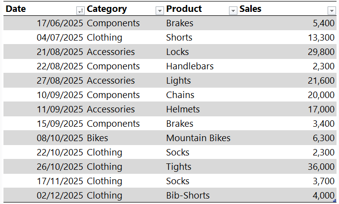
Let’s say I want to find the sales for this month. I can use this formula where cell D27 contains the current date:
=SUMIFS(Sales[Sales],
Sales[Date],">="&EOMONTH(D27,-1)+1,
Sales[Date],"<="&EOMONTH(D27,0))
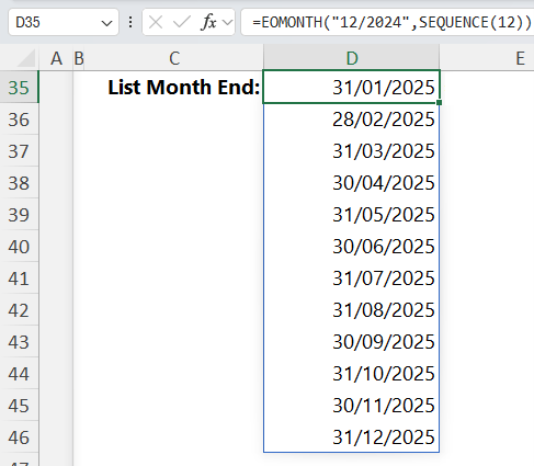
Or what if I want a list of month end dates? I can use EOMONTH with SEQUENCE to generate a list with this formula:
=EOMONTH("12/2024", SEQUENCE(12))
In the image below, you can see the result - a spilled array of month end dates for 2025:
🎓Get up to speed with EOMONTH here.
WORKDAY.INTL
Calculates working days while excluding weekends and holidays.
WORKDAY.INTL syntax:
WORKDAY.INTL(start_date, days, [weekend], [holidays])
Let’s say
I want to calculate the date 5 working days from Jan 2, 2025. My weekend days are Saturday and Sunday and I have a holiday on 6th Jan that I want to skip. I can use this formula:
=WORKDAY.INTL(DATE(2025,1,2), 5, 1, DATE(2025,1,6))
And it returns 10th
January 2025.
But that’s not all you can do with WORKDAY.INTL, it’s also super handy for returning a list of dates for building schedules etc.
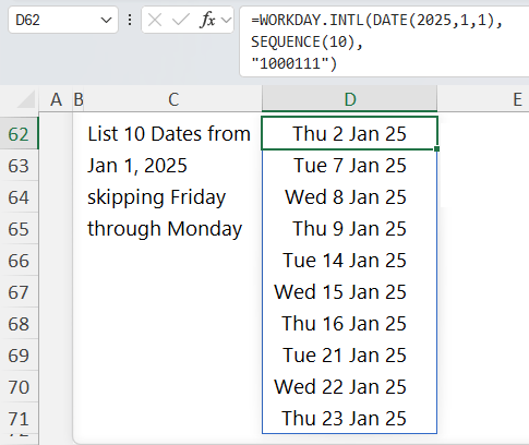
Let’s say I want a list of 10 dates from 1st Jan 2025, skipping Friday through Monday, because we deserve a super long weekend each week. I
can use this formula:
=WORKDAY.INTL(DATE(2025,1,1), SEQUENCE(10), "1000111")
Tip: notice the last argument in the formula above is a string of 1s and 0s. Instead of choosing from the built in weekends, I can specify the working days
with a 1 for days off and 0 for working days. We start with a 1 for Monday, which is a day off, then zeros for the workdays: Tuesday, Wednesday and Thursday, then 1 for Friday, Saturday and Sunday which I have off.
And we get a spilled array of our work dates:
🎓Get up to speed with WORKDAY.INTL here.
5. Custom Functions with LAMBDA – Build Your Own Tools
The LAMBDA function lets you create reusable, named formulas that behave like built-in functions. This is perfect for standardising and simplifying calculations across your organisation.
LAMBDA Syntax:
LAMBDA(parameter1,parameter2,..., calculation)
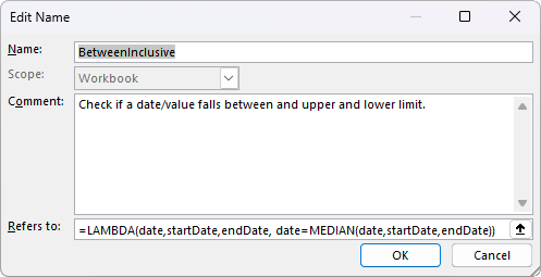
Example – sometimes we need to check if a date or value falls within a start/end date or upper and lower limit, but there’s no BETWEEN function in Excel, however we can use LAMBDA to create one:
=LAMBDA(date,startDate,endDate, date=MEDIAN(date,startDate,endDate))
You need to define the function as a name (Formulas tab > Define Name), I’ll call it BetweenInclusive because it checks if a date is within or equal to the start and end dates:
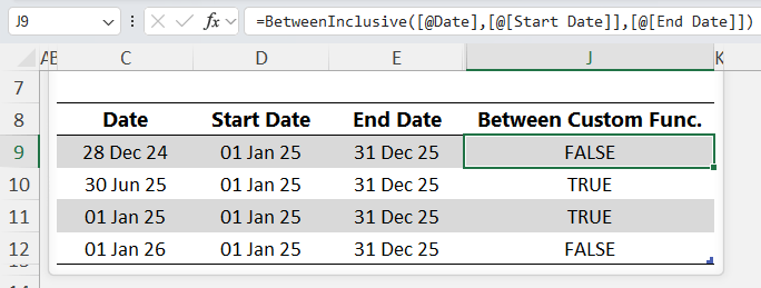
Once defined, you can call the function like any other:
=BetweenInclusive([@Date],[@[Start Date]],[@[End Date]])
🎓Get up to speed with LAMBDA here.
Next Steps
Mastering these 10 Excel functions: XLOOKUP, FILTER, SORT, UNIQUE, IF, SUMIFS, COUNTIFS, EOMONTH, WORKDAY.INTL, and LAMBDA, will transform the way you work with data. They cover the majority of real-world scenarios, from quick lookups and logic tests to advanced reporting and scheduling.
Ready to take your
skills even further?
👉 Explore my Excel courses here and learn how to combine these functions into smart, automated solutions that will set you apart in your
career.