If you’ve ever wasted time reformatting data, copying formulas,
or fixing PivotTables that mysteriously miss your latest data, you’re probably using plain cell ranges instead of Excel Tables.
Excel Tables aren’t just a visual upgrade - they’re a powerful feature that makes your spreadsheets dynamic, self-maintaining, and far less error-prone.
In this guide, you’ll learn:
How to create an Excel Table in seconds
The top benefits of Excel Tables over normal ranges
An Excel Table is a structured range of data that comes with built-in formatting, auto-expansion, structured references, and other features designed to make your work faster and more reliable.
How to Create an Excel Table
There are two easy ways:
Keyboard shortcut: Press Ctrl + T (it’s easy to remember ‘T’ for Table).
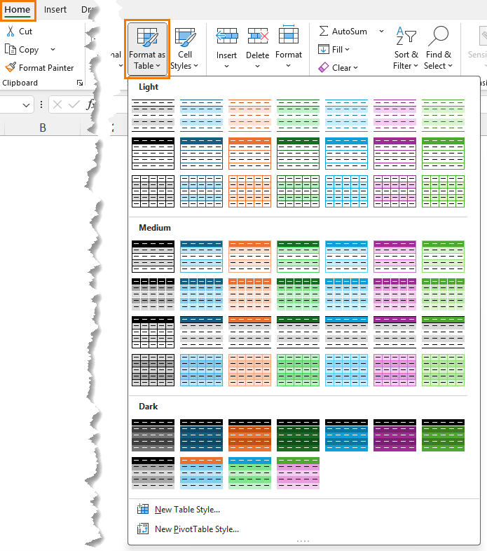
Menu: Go to Home → Format as Table, pick a style, tick My table has
headers, and click OK.
Your range is now an
official Excel Table - and that’s where the magic begins.
11 Reasons to Use Excel Tables
Here’s how Excel Tables solve the most common spreadsheet headaches:
1. Automatic Expansion for New Data
When you type in the row immediately below your table, or tab from the
last cell, it expands automatically - keeping formatting and formulas both inside and referencing the table inclusive of all data.
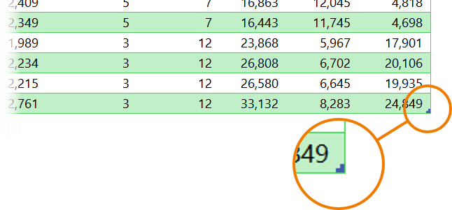
You can see the last cell in your table range denoted by the pull handle:
You can use this pull handle to resize the table manually if required.
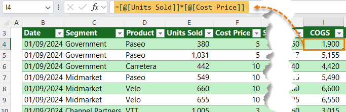
2. Readable Formulas with Structured References
Instead
of:
=E4*F4
You get formulas that use the column names:
=[@[Units Sold]] * [@[Cost Price]]
This makes formulas self-documenting and easier to debug.
3. Auto-Fill Formulas
Write a formula once, and Excel fills it down for you.
Override a single cell if needed - Excel will ask if you want to keep the change, however it’s recommended you keep formulas consistent within a column to avoid errors.
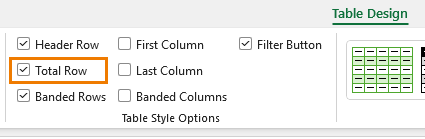
4. Built-In Total Row
Turn on Total Row in the Table Design tab for instant SUM, AVERAGE, COUNT, MAX, or MIN values.
Totals adjust automatically when you filter.
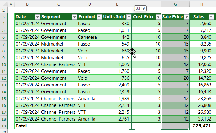
5. Drag-and-Drop Column Reordering
Just click and drag the
column header - formulas, totals, and formatting move with it. For example, in the image below I’m moving the Sale Price column to in between the Units Sold and Cost Price columns and you can see the vertical green line placeholder indicating where the column will be inserted:
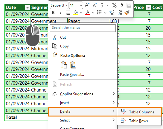
6. Safe Column Deletion
Right-click → Delete Table Columns - no risk of deleting unrelated data.
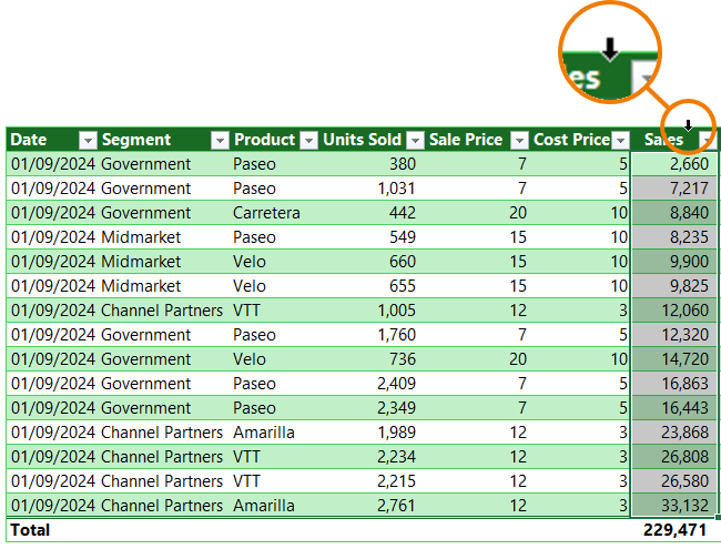
7. One-Click Column Selection
Hover over a header’s top edge, click the black arrow, and the whole column is selected - perfect for large datasets.
Use this technique for selecting data and when writing formulas for quick
authoring.
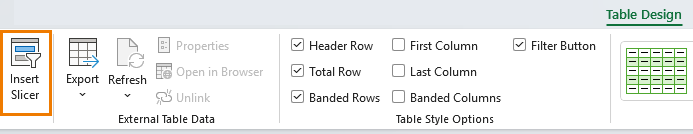
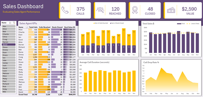
8. Visual Filtering with Slicers
Add Table Slicers for clickable, dashboard-style
filtering:
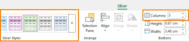
Go to Table Design → Insert Slicer
Choose the columns you want Slicers for
Increase the number of columns to arrange the buttons horizontally & customise colours and styles
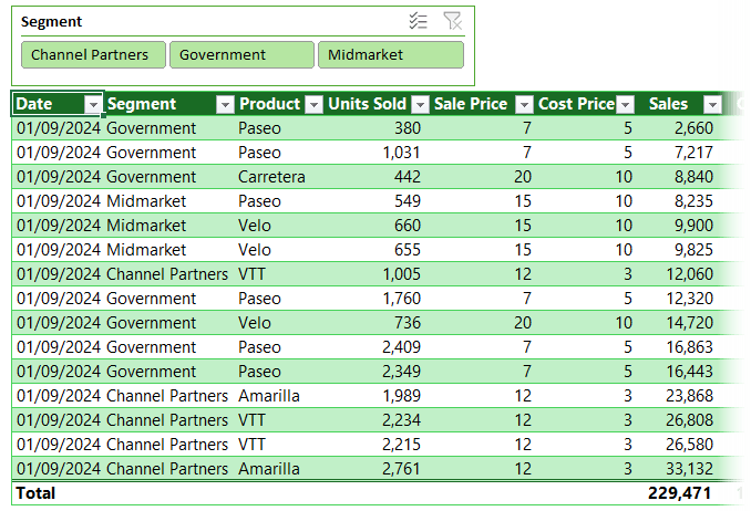
It’s like giving your table a built-in dashboard:
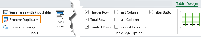
9. Remove Duplicates Instantly
Table Design → Remove Duplicates, pick your columns, and click OK. No
formulas or conditional formatting needed.
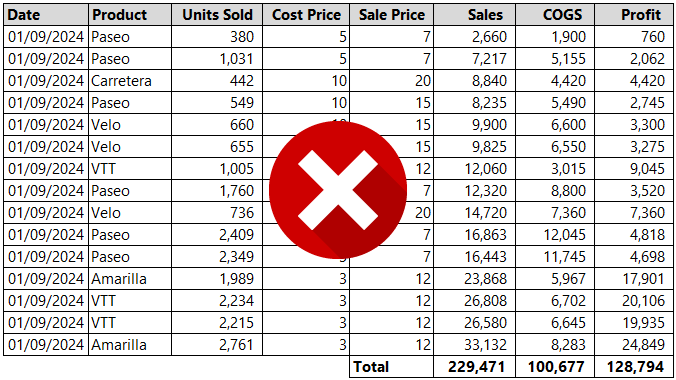
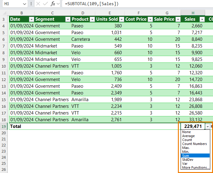
10. Dynamic Ranges in Formulas
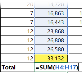
In a regular range, you add a few rows and suddenly your formulas aren’t picking them up – as you can see below, the last row that was just added is not included in the original SUM formula:
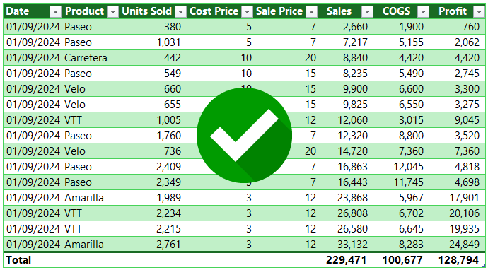
Tables solve that. When you use the Table’s structured references, Excel always includes the full column range - no matter how much your data grows.
So instead of writing:
=SUM(H4:H1000)
You type the reference: TableName[ColumnName] (or use the mouse to click the column you want and have Excel insert the table structured reference for you):
=SUM(Table1[Sales])
And it just works. Even when your 1000 rows become 10,000.
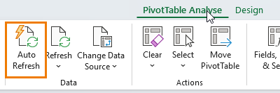
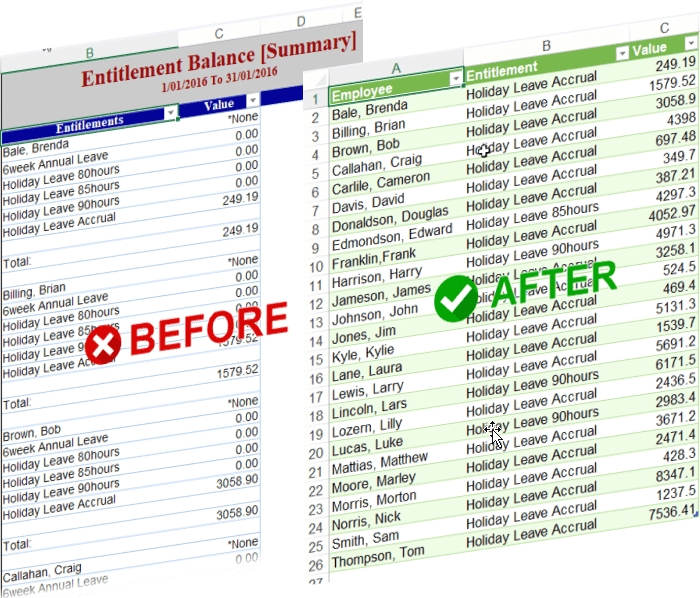
11. PivotTables That Always Stay Updated
PivotTables based on Tables auto-expand to include new rows. Just right-click and refresh to update the PivotTable - or in
Microsoft 365, enable auto-refresh for hands-free updates.
Pro-Level Excel Table Tips
Once you’re comfortable with Tables, try these advanced tricks:
1. Clean and Transform Data with Power Query
Load your Table into Power Query (Data → From Table/Range) to clean messy data automatically. Then refresh it with a single click.
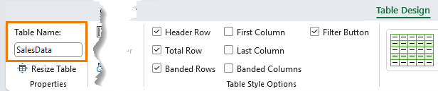
Rename it to SalesData – on the Table Design tab in the ‘Table Name:’ box:
Now you can write your formulas without even using the mouse:
=SUM(SalesData[Profit])
Plus, it’s cleaner and easier to manage
across multiple sheets.
Why Switch to Excel Tables?
Using Tables means:
No more broken formulas when adding rows
Instant totals and filters
Clean, readable
formulas
Dashboards and PivotTables that stay in sync with your data
If you’re still using plain ranges, now’s the time to make the switch.
Next Step
Build your next dataset as an Excel Table and see how much time you save. And if you’re ready to take Excel even further, explore my Excel & Power BI courses for step-by-step training that turns good spreadsheets into great ones.
Want to sponsor our newsletters? Just reply to this email to get in touch with us.
Learn With Us
This email may contain affiliate links. This means I may earn a commission should you choose to make a purchase using my link. But we only promote courses we believe will benefit you.