Hi ,

If you’ve ever tried to track your spending in Excel but gave up because it took too long to enter transactions manually… this guide is for you.

In this tutorial, I’ll show you how to build an automated personal finance tracker in Excel that lets you simply import or paste your bank transactions, and then Excel automatically:

• Classifies every transaction
• Updates your savings goals
• Refreshes your dashboard
• Shows your financial progress in one clean, visual summary

Plus, it includes a fully integrated Savings Goals tracker that automatically allocates your savings, calculates remaining balances, and estimates how many months you’ll need to reach each goal.

This is the perfect project to kick off the year with control, clarity, and confidence.

Note: Works best with Microsoft 365 or Excel 2021 onward (for the dynamic array formulas used in the Schedule view). However, the Tracker itself works in older versions too. 

Prefer to read this on our website? 

Then click this link >>> Automated Personal Finance Tracker

Video: Automated Personal Finance Tracker

Watch on YouTube

What You’ll Learn in This Tutorial

• How to build a Transactions Table that automatically categorises your data
• How to create a Category Mapping Table for instant classification
• How to cleanly organise your data with structured references
• How to prepare your workbook for dashboards and PivotTables
• How to create a savings goal tracker that automatically udpates

Let’s get started with the Transactions sheet — the heart of your tracker.

1. Create the Transactions Table

Your Transactions sheet is the only place you’ll ever paste data from your bank.

No manual entry. No typing. No double-handling.

1.1 Insert Your Transactions Sheet

1. Insert a new worksheet
2. Rename it Transactions

1.2 Create Your Table Headers

Enter the following headers:

• Account
• Date
• Description
• Debit (Spend)
• Credit (Income)
• Income/(Expense)
• Subcategory
• Category
• Category Type

1.3 Convert to an Excel Table

Select the headers, then:

Home tab → Format as Table:

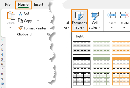
Tick “My table has headers”:

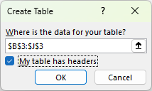
Rename the table to:

tblTrans (Table Design → Table Name)

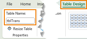
This ensures formulas fill automatically and PivotTables always expand.

2. Import or Paste Your Bank Transactions

Here’s where your time savings begin.

Instead of typing transactions manually, simply:

1. Download your bank statement (CSV, Excel, or copy from your banking app)
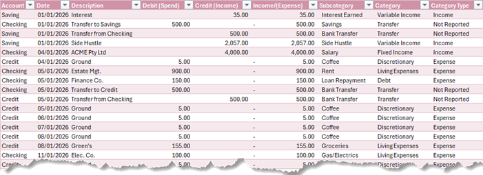
2. Paste directly into tblTrans under:

• Account
• Date
• Description
• Debit (Spend)
• Credit (Income)

Debits represent money going out.
Credits represent money coming in.

We will take care of the rest with formulas.

3. Add the Income/(Expense) Formula

To make analysis easier, we convert Debit and Credit into a single “net impact” column.

In the Income/(Expense) column, first data row (inside the table), enter:

=[@[Credit (Income)]] - [@[Debit (Spend)]] 

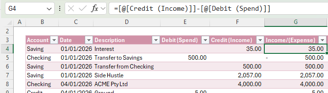
This gives:

• Positive numbers for income
• Negative numbers for spending

Because this is inside a table, Excel auto-fills down instantly.

4. Build the Category Mapping Table

To classify each transaction automatically, we use a simple lookup table.

4.1 Create a New Sheet

Insert a new worksheet and name it Category Table.

4.2 Add Category Headers

Enter the following headers:

• Description
• Subcategory
• Category
• Category Type

Convert this range to a table and rename is tblCat

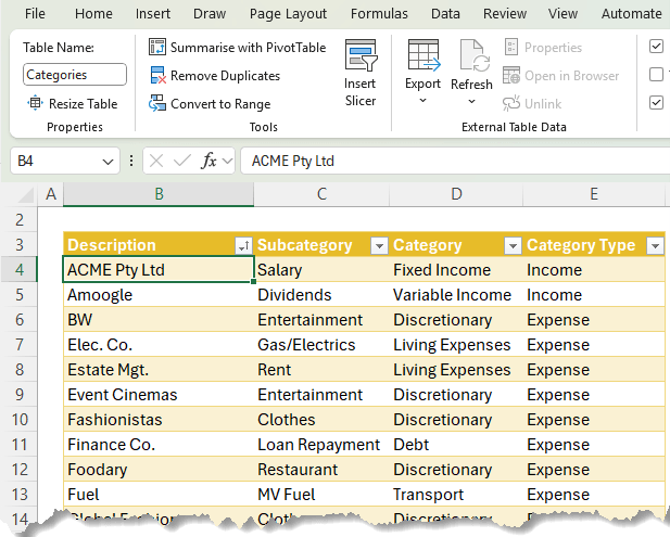
4.3 Enter Your Mapping Rows

Fill in key words that appear in your bank transaction descriptions and map each to a category:

Tip:
You don’t need to type full bank descriptions — just a distinctive keyword.

Excel will search for that keyword inside each transaction’s Description column.

5. Automatically Classify Transactions with XLOOKUP

Now return to your Transactions sheet.

We’ll use a combination of SEARCH, ISNUMBER, and XLOOKUP to detect keywords and automatically classify the transactions.

5.1 Subcategory Column

In the Subcategory column, first data row:

=XLOOKUP(
    TRUE,
    ISNUMBER(SEARCH(Categories[Description],[@Description])),
    Categories[Subcategory],
    "Uncategorised"
    )
                                                            

This formula classifies each transaction by Subcategory based on the text in its Description.

The Categories table contains “keywords” in Categories[Description] and the corresponding Categories[Subcategory].

So the logic is:

“Look through the list of Description keywords and find the first one that appears anywhere inside this transaction’s Description. When you find it, return the matching Subcategory. If nothing matches, return ‘Uncategorised’.”

SEARCH performs and array calculation that tries each keyword in Categories[Description] inside the string [@Description].

The result is an array of numbers and errors, one per row in Categories[Description], where:

• Number = keyword was found (position in the text).
• #VALUE! error = keyword not found.

We wrap SEARCH in ISNUMBER which takes that array of numbers and errors and converts it into TRUE/FALSE:

• ISNUMBER(1) → TRUE
• ISNUMBER(#VALUE!) → FALSE

So now you have an array like:

{FALSE; FALSE; TRUE; FALSE; ...}

This tells you, for each row in Categories, whether that 

keyword is present in the transaction description.

We then use XLOOKUP to scan down the lookup_array and look for the first TRUE:

=XLOOKUP(
    TRUE,   // lookup_value
   
ISNUMBER(SEARCH(...)), // lookup_array → {FALSE; FALSE; TRUE; ...}
    Categories[Subcategory], // return_array  "Uncategorised"// if_not_found
    ) 
                                                            

Once XLOOKUP finds the first TRUE, it returns the corresponding item from Categories[Subcategory] (the return_array).

If no keyword in Categories[Description] appears in the transaction Description, then SEARCH(...) returns only errors, ISNUMBER(...) returns only FALSE values, and XLOOKUP doesn’t find any TRUE.

In that case, XLOOKUP returns the if_not_found argument: “Uncategorised”.

So, any description you haven’t yet added to the Categories table shows up as Uncategorised, making them easy to filter and classify later.

5.2 Category Column

We then copy the formula to the Category column and change the return array to the ‘Category’:

=XLOOKUP(
    TRUE,
    ISNUMBER(SEARCH(Categories[Description],[@Description])),
    Categories[Category],
    "Uncategorised"
    ) 

5.3 Category Type Column

Copy the formula again and change the return array to the ‘Category Type’ column:

=XLOOKUP(
    TRUE,
    ISNUMBER(SEARCH(Categories[Description],[@Description])),
    Categories[Category Type],
    "Uncategorised"
    ) 

Result:
Every time you paste new transactions, Excel instantly classifies every row.

No manual categorisation. No data cleanup.

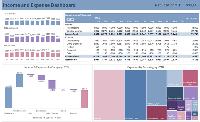
6. Building the Dashboard: Your Year-to-Date Money Story at a Glance

With your data and categories set up, the dashboard transforms hundreds of rows of transactions into a clean, visual overview of:

• Income by month
• Expenses by month
• Net income
• Spending by category
• A waterfall breakdown of where your money goes
• Savings goal progress

All charts and metrics update with a single click.

The dashboard uses:

• PivotTables for summarising your data
• Column charts for Income, Expenses and Net Position
• A Waterfall chart for understanding how each category influences your overall results
• A Treemap for visualising category spend as a proportion of total expenses
• A Donut chart for savings progress

Each visual is built intentionally to help you spot patterns faster and understand the story behind your spending.

7. PivotTables: The Engine Behind the Insights

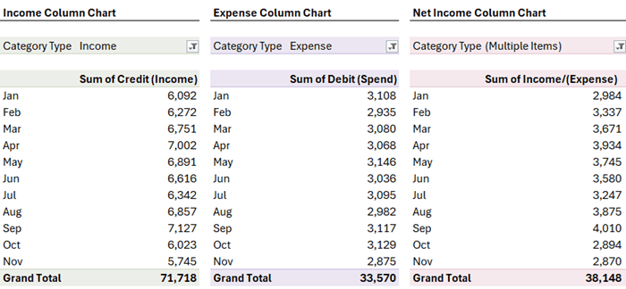
The dashboard is powered by several PivotTables located on an Analysis sheet. The PivotTables for the Total Income, Total Expenses and Net Income charts are shown below:

Watch the video for step-by-step instructions for building the PivotTables.

Monthly Income PivotTable

Filters by Category Type = Income, groups dates by month/year, and sums the Credit column.

Monthly Expense PivotTable

Filters by Category Type = Expense, and sums the Debit column.

Net Income PivotTable

Combines both income and expense using the Income/(Expense) column.

Profit & Loss PivotTable

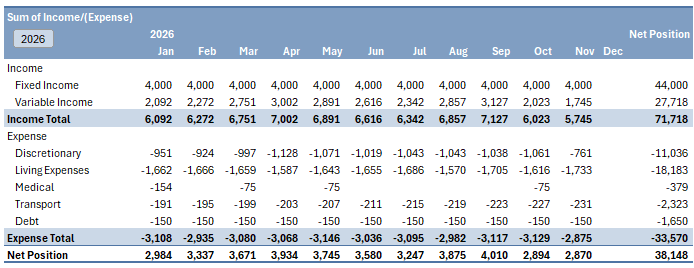
This PivotTable breaks down your income and expenses by category and month so you can:

• Compare fixed vs discretionary spending
• Spot unusually high months
• Understand your true net position year-to-date

This P&L becomes the starting point for your Waterfall chart.

Waterfall Chart: Where Your Money Really Goes

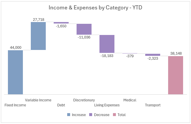
The Waterfall chart is ideal for answering the question:

“What categories contribute the most to my financial position?”

It gives you a running total of income vs expenses across categories, making overspending stand out instantly.

Treemap Chart: The Fastest Way to Compare Category Spending

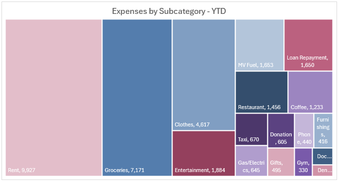
While the Waterfall shows direction (adds/subtracts), the Treemap shows proportion.

It helps you quickly see:

• Which category is your biggest expense
• Which areas are growing over time
• How discretionary vs essential spending compares

The Waterfall and Treemap charts don’t accept PivotTables as their source data, so:

1. Copy the PivotTable
2. Paste it as values
3. Insert a Treemap
4. Re-point the source to the PivotTable cells

The result is a bold visual snapshot of your spending structure linked to dynamic PivotTables for automatic updates.

8. Savings Goals: Automatically Allocate Your Savings by Priority

One of the best parts of this model is the Savings Goals sheet: it takes your overall savings balance and automatically allocates it to your goals in order of priority. No manual juggling of numbers.

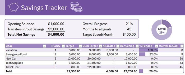
8.1 Set up the Savings Summary

Insert a new sheet for the Savings Goals, start with a small summary block at the top.

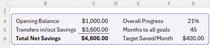
Add headings

• Opening Balance
• enter your current savings balance (e.g. 1000)
• Transfers in/out Savings
• Total Net Savings

You’ll also set up a couple of summary labels on the right (we’ll use them later):

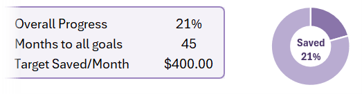
• Overall Progress
• Months to all goals
• Target Saved/Month

Calculate transfers into/out of savings

In C5, enter:

=-SUMIFS(tblTrans[Income/(Expense)], tblTrans[Subcategory], "Savings")

• This sums all Income/(Expense) values where Subcategory = "Savings".
• The leading minus sign converts the net effect into a positive “amount added to savings”.

Total net savings available for goals

In C6, enter:

=SUM(C4:C5)

This is your Total Net Savings: opening balance plus net transfers.

Now give C6 a named range:

• Select C6 → Formulas → Define Name → Name: TotalSavings.

8.2 Create the Savings Goals Table

Next, create a table for your individual goals.

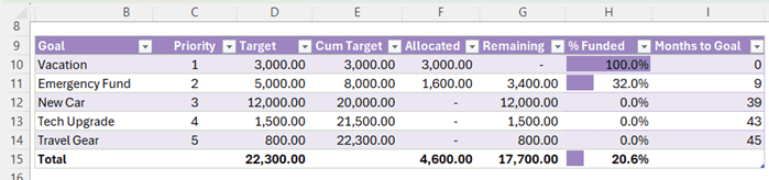
Below these headers (rows 10 onward), enter your goals, priorities (1 = highest priority), and target amounts, for example:

• Vacation, Emergency Fund, New Car, Tech Upgrade, Travel Gear, etc.

Turn it into a Table

• Select B9:I (including the headers and your goal rows).
• Insert → Table → tick “My table has headers”.
• Name the table tblGoals (Table Design → Table Name).
• Turn on the Totals Row for tblGoals (Table Design → Total Row).

8.3 Cum. Target – Cumulative target by priority

The Cum. Target column adds up all target amounts up to each priority level.

Cum. Target formula

In E10 (first data row of Cum Target inside tblGoals), enter:

=SUMIFS([Target], [Priority], "<=" & [@Priority]) 

• [@Priority] is the priority of the current row.
• The formula sums all Target values where Priority ≤ current Priority, giving you a running total of your targets by priority.

8.4 Allocated – Allocate savings by priority

Now we tell Excel how much of your TotalSavings goes to each goal, based on its priority and the cumulative targets.

Allocated formula with LET function

In F10 (first Allocated row), enter:

=LET(
    total,  TotalSavings,
    prev,   [@[Cum Target]] - [@Target],
    avail,  total - prev,
    MAX(0, MIN([@Target], avail))
    )

What this does:

• total = the named range TotalSavings (cell C6) – the total savings to allocate.
• prev = cumulative target before this goal (Cum Target – Target).
• avail = what’s left after funding all higher-priority goals (total - prev).
• MIN([@Target], avail) = the smaller of:
  • the goal’s target, and
  • the savings available for this goal.
• MAX(0, …) ensures we never allocate a negative amount.

You’ll see that the total of the Allocated column matches TotalSavings, spread across goals in priority order.

8.5 Remaining and % Funded

Remaining amount

In G10, enter:

=[@Target] - [@Allocated] 

This shows how much is still needed for each goal.

% Funded

In H10, enter:

=IF([@Target]=0, 0, [@Allocated]/[@Target]) 

Copy down.

• If a goal has no target, it returns 0.
• Otherwise, it returns the fraction of the goal that’s funded.

You can then apply Conditional Formatting → Data Bars to the % Funded column for a quick visual progress bar, and adjust the colour to match your theme.

8.6 Months to Goal

To estimate how many months it will take to reach each goal, you’ll set a monthly savings target and use that in the formula.

Target Saved/Month

In G6, enter your planned monthly savings amount (for example, 400), next to the label in E6: Target Saved/Month.

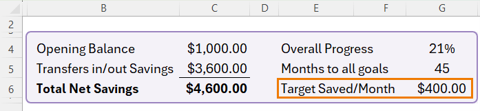
Then define a name:

• Select G6 → Formulas → Define Name → Name: TargetSavedMonthly.

Months to Goal formula

In I10, enter:

            =IF(TargetSavedMonthly<=0,"",
    MAX(0, ROUNDUP(([@[Cum Target]] - TotalSavings) / TargetSavedMonthly, 0)
        )
        )
                                           

Explanation:

• If TargetSavedMonthly is 0 or less, the formula returns an empty string (no calculation).
• Otherwise, it:
  • Takes Cum Target – TotalSavings (how much you still need to have saved overall by this point),
  • Divides by your monthly savings target,
  • Rounds up to whole months, and
  • Wraps it in MAX(0, …) so you don’t see negative months if you’re already ahead.

This gives a realistic “months remaining” estimate for each goal, based on your current savings and how much you plan to save each month.

8.7 Summary Metrics in the Header

Finally, link the goals table back to the header summary so you can chart overall progress.

Overall progress

In G4, enter:

=tblGoals[[#Totals],[% Funded]] 

This pulls the Total row of % Funded from tblGoals.

In H4, enter:

=1 - G4

You can now select G4:H4 and insert a Doughnut chart to visualise the proportion of your total goals that’s funded vs unfunded.

See video for the doughnut chart step-by-step.

Months to all goals

In G5, enter:

=MAX(tblGoals[Months to Goal]) 

This returns the largest “Months to Goal” value,  i.e. how long it will take to complete all goals at your current monthly savings rate.

With this Savings Goals tracker in place, your dashboard shows where your money went and how close you are to the things you actually care about: trips, emergency funds, a new car, or anything else you’re saving for.

9. Keeping the Model Updated: One Step, Zero Rework

Updating this tracker is designed to be effortless.

Whenever you want to refresh the report:

1. Download or copy your latest bank transactions
2. Paste them into the next empty row of the Transactions table
3. Fix any uncategorised descriptions by adding them to the Category Table
4. Press Refresh All

All calculations, PivotTables, charts, and your Savings Goals update automatically. No formulas to adjust, no charts to rebuild.

Final Thoughts

This system gives you total clarity:

• Where your money is going
• How much you're saving
• Whether you're on track for your goals
• How your spending is trending month-to-month

Use it weekly or monthly, and you’ll always know your financial position at a glance.

Automate Getting Bank Transactions

If you want to take this tracker to the next level, the smartest upgrade is automating the bank-transaction import. Instead of copying and pasting, Power Query can fetch and clean your data for you. Get started with Power Query here.

Have a great day,

Mynda Treacy

Co-founder My Online Training Hub

Want to sponsor our newsletters?  Just reply to this email to get in touch with us.