Hi ,

If you’ve ever lost track of what’s due, this post walks you step-by-step through building a clean Excel Assignment or Task Tracker.  

You’ll set up validated drop-downs, an automatic Days Available countdown, colour-coded Status:

And a simple calendar-style schedule, all with standard Excel features.

Note: Works best with Microsoft 365 or Excel 2021 onward (for the dynamic array formulas used in the Schedule view). However, the Tracker itself works in older versions too. 

Prefer to read this on our website? 

Then click this link >>> Excel Assignment/Task Tracker

Video: Excel Assignment/Task Tracker

Watch on YouTube

1) Create the Lists (for drop-downs)

1. Insert a sheet named Lists.

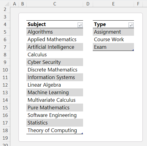
2. In C4, type Subject, then list your subjects in C5:C18 (e.g., Algorithms, Applied Mathematics, Artificial Intelligence, …, Theory of Computing).

3. In E4, type Type, then list Assignment, Course Work, Exam in E5:E7.

4. Turn each list into a Table so new items auto-extend:

• Select C4:C18 → Ctrl+T → My table has headers → OK → Table Design → Name: Subjects
• Select E4:E7 → Ctrl+T → Name: Types

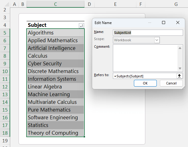
5. Create named ranges for clean validation:

• Formulas > Name Manager > New
  • Name: SubjectList → Refers to: =Subjects[Subject]

• Repeat for the Work Types:
  • Name: WorkTypes → Refers to: =Types[Type]

Why this matters: As you add subjects or work types later, your drop-downs will automatically include them.

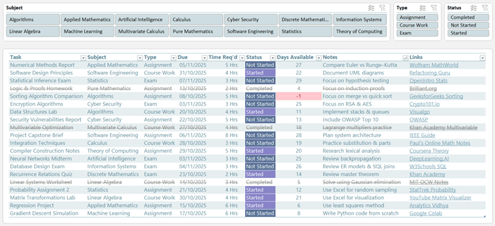
2) Build the Tracker Table

1. Insert a sheet named Tracker.

2. In C7:K7 enter these headers (or modify as required to your own needs):
Task | Subject | Type | Due | Time Req’d | Status | Days Available | Notes | Links

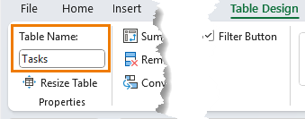
3. Convert the range to a Table: select one header cell → Ctrl+T → My table has headers → OK → Table Design → Name the table via the Table Design tab: Tasks.

4. Add data validation:

• Select the Subject column (D): Data > Data Validation > List → Source: =SubjectList
• Select the Type column (E): List → Source: =WorkTypes
• Select the Status column (H): List → Source (type in the list separated by commas):
  1. Not Started,Started,Completed

5. Days Available formula (counts down to the due date):

• In the first data row of Days Available (cell I8):

=[@Due]-TODAY()

Press Enter and Excel will fill it down the table.

Tips: Set your preferred date format on the Due column (Ctrl+1). Keep Notes and Links columns wide enough for readability.

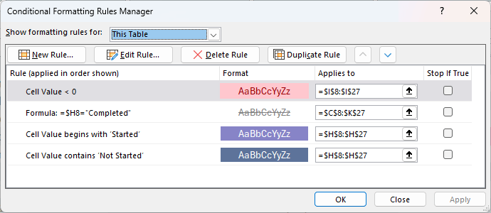
3) Conditional Formatting (make the tracker “readable at a glance”)

A) Highlight overdue tasks

1. Select the Days Available column cells (column I).

2. Home > Conditional Formatting > Highlight Cells Rules > Less Than…

3. Type: 0 → choose a light red fill with dark red font.

B) Colour the Status values

1. Select the Status column cells (column H).

2. Home > Conditional Formatting > New Rule > Format only cells that contain

• Specific Text → Containing → Not Started → choose a clear “attention” fill.
• Specific Text → Begins with → Started → choose an in-progress amber.

C) Strike through completed rows (entire row)

1. Select the entire Tasks table (click inside → Ctrl+A).

2. Home > Conditional Formatting > New Rule > Use a formula to determine which cells to format

3. Enter a formula that checks your Status column (adjust the letter to your sheet; e.g., if Status is in column I):

=$H8="Completed"

4. Format… → set Font color to light grey and Strikethrough → OK → OK.

Note: The dollar sign locks the column (Status) while the row changes per record.

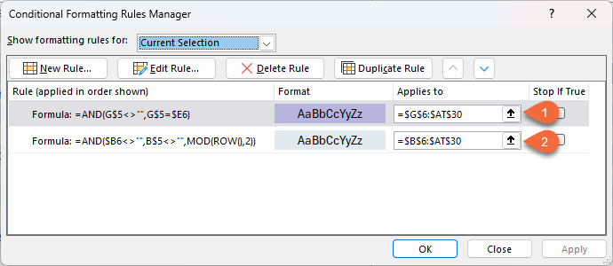
You should have the following rules:

4) Add Slicers (fast filtering)

1. Click anywhere in the Tasks table.

2. Table Design > Insert Slicer → tick Subject, Type, Status → OK.

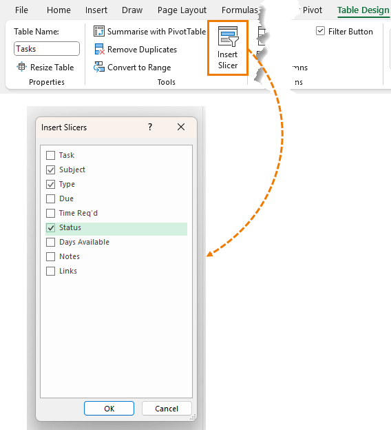
3. Arrange the slicers near the table. (Optional: apply your custom slicer style and tweak sizes/columns for a clean layout.)

Result: You can instantly focus on a single subject, filter to “Exam”, or only show “Not Started”.

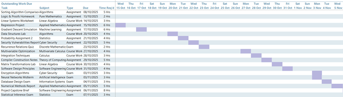
5) Build the Schedule View (mini calendar)

This gives you a compact, calendar-style overview that updates automatically.

1. Insert a sheet named Schedule.

2. In B5:F5, add headers (customise as required): Task | Subject | Type | Due | Time Req’d.

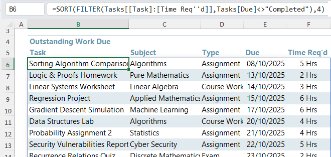
A) Spill a sorted list of active (not completed) tasks

In B6, use the SORT and FILTER functions:

=SORT(
                  FILTER(Tasks[[Task]:[Time Req'd]], Tasks[Status]<>"Completed"), 4)

This pulls columns Task through to Time Req’d for tasks not completed and sorts by the 4th column in that slice (Due date).

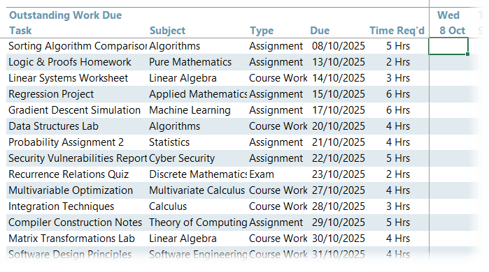
B) Create a horizontal row of dates

In G5, use the SEQUENCE function to automatically generate the date range your tasks span:

=SEQUENCE(, MAX(Tasks[Due]) - MIN(Tasks[Due]) + 1, MIN(Tasks[Due])) 

• Spills dates across (one column per day) from the earliest to the latest due date.

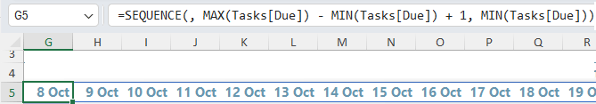
Optional day-of-week row above (in G4):

=G5#

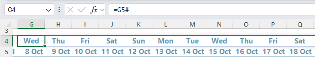
Format G4 as ddd (Mon, Tue, …) and G5 as d mmm (1 Jan).

C) Banded rows for readability (since spilled array formulas can’t be inside Tables)

1. Select a generous output region beneath the headers to allow for more tasks and more dates, e.g., B6:AT30.

2. Home > Conditional Formatting > New Rule > Use a formula to determine which cells to format

3. Use:

=AND($B6<>"", B$5<>"", MOD(ROW(),2)) 

Choose a soft fill colour.

Why this works: It only bands rows with data and columns with headers/dates, and it alternates rows with MOD.

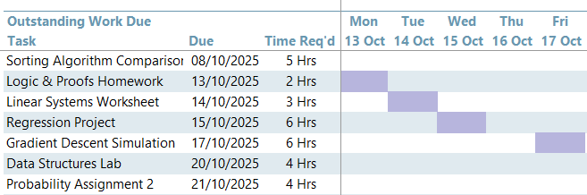
D) Mark each task’s due date on the timeline

1. Select the date grid area (e.g., G6:AT30).

2. Conditional Formatting > New Rule > Use a formula

3. Use:

=AND(G$5<>"", G$5=$E6) 

This highlights the cell where the column header date equals the row’s Due date (E).

1. Pick a strong highlight fill.

2. Note: in Conditional Formatting > Manage Rules, move this date-highlight rule above the banded rows rule so it isn’t overridden.

E) Finishing touches

• View > Freeze Panes at G6 to keep task info visible while you scroll the date grid.
• View > Show > Gridlines off for a cleaner dashboard look.

You’re done!

You’ve built a reusable, no-macro tracker with:

• Clean data entry via drop-downs
• A live Days Available countdown (overdue flags included)
• Quick filtering with Slicers

• A dynamic Schedule view that updates as your table changes

Upgrade Your Skills

If you’d like a broader toolkit so projects like this feel effortless, our Excel Expert Course is designed to give you a wide range of professional-grade skills you can apply to any workbook. Plus, it includes support and mentoring personally from Microsoft MVP, Mynda Treacy.

Have a great day,

Mynda Treacy

Co-founder My Online Training Hub

Want to sponsor our newsletters?  Just reply to this email to get in touch with us.