What Is the HYPERLINK Function?
Excel’s HYPERLINK function lets you create clickable links, not just for web pages, but also for internal sheet navigation and file shortcuts.
Syntax:
=HYPERLINK(link_location, [friendly_name])
- link_location: The destination URL, file path, or cell reference.
- friendly_name: [Optional] The text you want displayed (instead of the raw link).
1. Clean Up Messy URLs in Reports
If your reports are filled with long, ugly URLs like this:
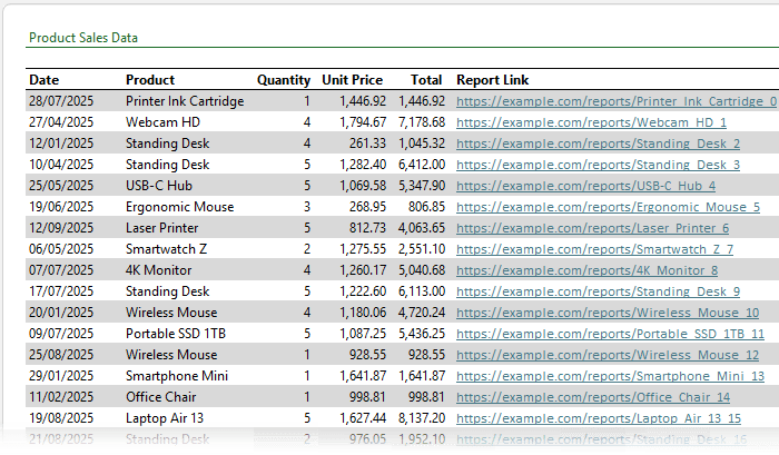
You can replace them with neat anchor text like “View Report” resulting in a cleaner, neater report free of clutter:
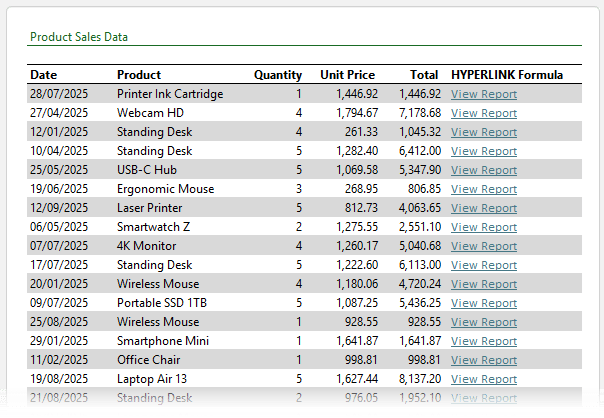
Formula:
=HYPERLINK([@[Report Link]], "View Report")
This formula
creates a clickable label while keeping the actual URL hidden in another column (which you can safely hide). It makes your reports look professional and much easier to read.
Pro Tip: Always test your links before sending the file to someone else. Excel won’t tell you if a URL is broken.
2. Build
a Table of Contents to Navigate Between Sheets
When your workbook has multiple sheets, clicking back and forth wastes time.
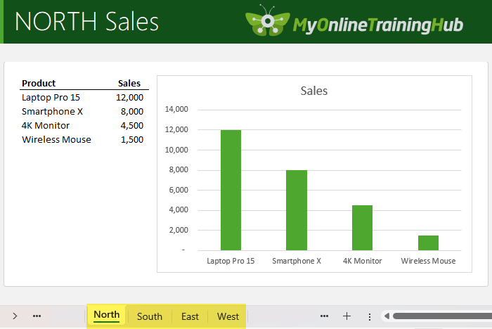
Instead, create a Table of Contents (TOC) sheet with clickable links to each tab.
Example:
=HYPERLINK("#"&C6&"!A1", C6&" Report")
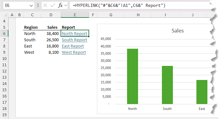
Here’s what’s happening:
- The # tells Excel it’s an internal link.
- C6 contains the sheet name (e.g. “North”).
- !A1 is the target cell within that sheet.
- The friendly name shows as “North Report”.
This technique helps others navigate your workbook without getting lost.
Bonus: You can also create
navigation buttons using shapes:
- Insert a rectangle → type the sheet name.
- Press Ctrl+K → “Place in This Document”.
- Select the sheet you want to link to.
- Repeat for all sheets.
- Colour code shapes to indicate which is the currently selected sheet.
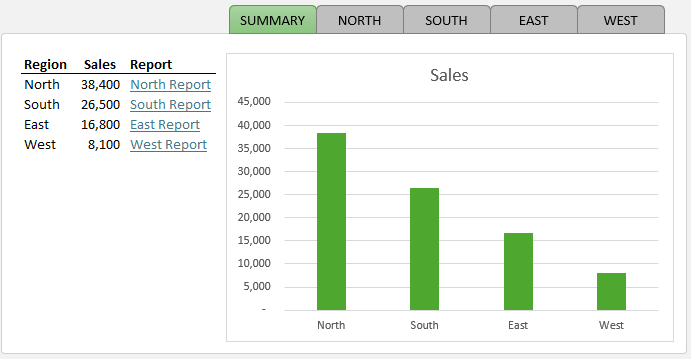
Tip: You can even hide the sheet tabs (File → Options → Advanced → Display options for this workbook) to make your dashboard look sleek and controlled.
3. Link Directly to Files and Folders
The HYPERLINK function isn’t just for websites — it can also open files or folders directly from Excel.
Examples:
=HYPERLINK("C:\Project Gemini\Specifications.pdf", "Customer Requirements")
=HYPERLINK("C:\Reports\", "Open Reports Folder")
This trick lets you create a single Excel hub for all project files. It’s perfect for teams that constantly share supporting documents, contracts, or images.
Note: Use OneDrive or SharePoint paths for shared workbooks so everyone can access the same links.
4. Create Dynamic Hyperlinks with XLOOKUP
You can even use formulas to create dynamic links that update based on a selection.
Imagine you have an order database and a dropdown list of Order IDs. You can use XLOOKUP to return details for the selected order and a HYPERLINK that jumps straight to the matching row:
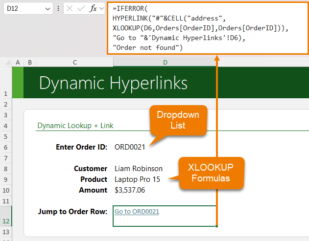
Formula:
=IFERROR(
             HYPERLINK("#"&CELL("address",
             XLOOKUP(D6,Orders[OrderID],Orders[OrderID])),
             "Go to "&'Dynamic Hyperlinks'!D6),
             >"Order not found")
How it works:
- XLOOKUP finds the matching Order ID and returns its cell reference.
- CELL("address", …) gets that cell’s
address.
- # makes it an internal link.
- The friendly name shows as “Go to [Order ID]”.
Clicking the link takes you directly to that order in your database. No scrolling, no searching.
Common Mistakes to Avoid
- Broken File Paths:
Excel doesn’t check whether the linked file actually exists. Always double-check your paths and test them before sharing. - Sheet Names
with Spaces:
If your sheet name includes spaces (e.g., Sales Data), wrap it in single quotes:
=HYPERLINK("#'Sales Data'!A1", "Open Sales Sheet")
Tip: It’s good practice to always include quotes, just in case.
Take It Further
If you love turning workbooks into interactive tools that do the work for you, you’ll love my Advanced Excel Formulas
Course.
You’ll master formulas like LET, LAMBDA, IFERROR, and XLOOKUP to automate workflows and eliminate repetitive manual steps.