The Problem with Lookup Formulas
Let’s say your boss asks for a sales report showing which products are selling best by region.
You’ve got all the data you need, but it’s spread across three tables:
- Sales Data (with 2,000+ transactions)
- Products (with product names, categories, and unit prices)
- Sales Reps (with regional details)
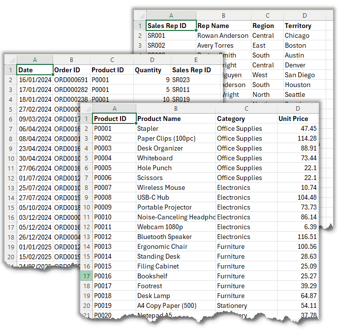
The sales data only shows cryptic Product IDs like
P0003 or P0015. So, naturally, you start building lookup formulas:
=XLOOKUP($C2, Products!A:A, Products!B:D, "")
This brings in the product name, category, and unit price. Add a formula to calculate the sales value:
=D2*H27
Soon, your file contains 8,000 formulas and 6,000 duplicated cells.
And the problems don’t stop there:
- Every time you add new data, you have to copy the formulas down.
- Performance slows as Excel recalculates thousands of lookups.
- Adding more tables (like Sales Reps) makes the formula mess even worse.
This isn’t just inefficient, it’s unsustainable.
The Solution: Think Like a Database with Power Pivot
The solution isn’t writing “better” lookup formulas. It’s re-thinking how data should be structured.
Instead of duplicating, you need to connect your tables. That’s exactly what Excel’s Power Pivot allows you to do.
Here’s how it works:
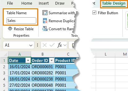
1. Convert each dataset into an Excel Table
- Select your data → Press Ctrl+T
- Rename them: Sales, Products, and Reps respectively
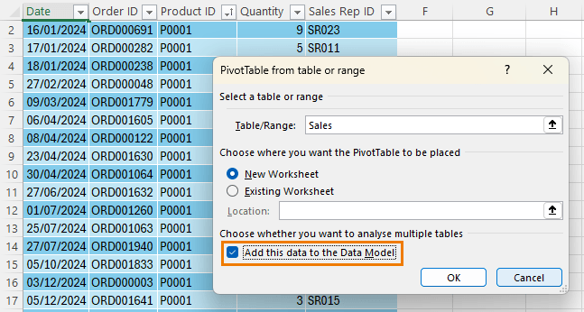
2. Add Tables to the Data Model
- Insert → PivotTable → Check Add this data to the Data Model
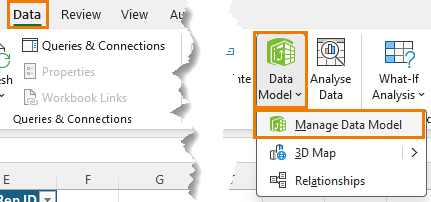
3. Define Relationships in Power Pivot
- Open Power Pivot via the Data tab > Data Model > Manage Data Model
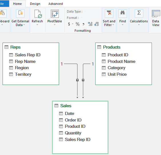
- Go to the Diagram view (Home tab):
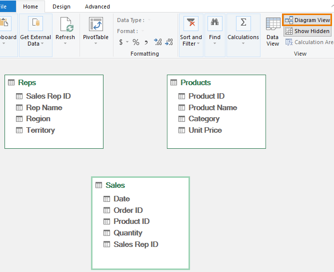
- Create relationships between the tables by left clicking and dragging the column names to each table as follows:
- Sales → Products via Product ID
- Sales → Reps via Sales Rep ID
Now, all your tables are connected behind the scenes:
Building PivotTables Without Formulas
With relationships set, you can build reports instantly using fields from any of the related tables:
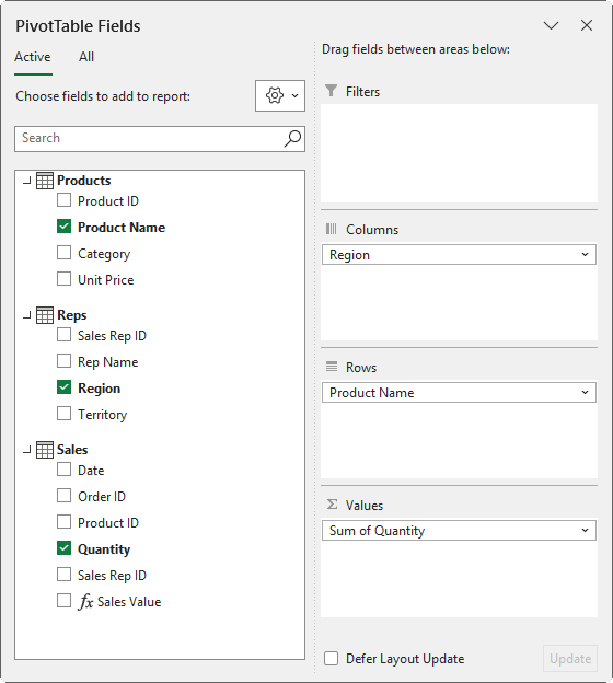
- Place Region from the Reps table in the
Columns
- Place Product Name from the Products table in the Rows
- Place Quantity from the Sales table in the Values
And just like that, you have a snapshot of your
products by region:
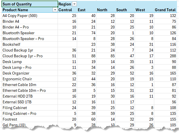
No lookups. No
duplication. No performance issues.
This is exactly how professional database systems work, and now you have that same power inside Excel.
Going Beyond Lookups With Measures
Power Pivot isn’t just about relationships. It also gives you DAX measures, which are formulas
that work directly inside PivotTables.
Insert a measure from the Power Pivot tab > Measures > New Measure:
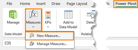
For example, to calculate Sales Value:
=SUMX(
Sales,
Sales[Quantity] *
RELATED(Products[Unit Price])
)
This single measure replaces thousands of row-level formulas.
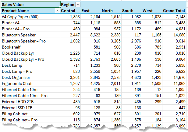
Instead of 2,000 formulas in your data table, the measure only calculates the 438 unique values needed in the PivotTable. Faster, cleaner, and far more efficient.
Why You Should Stop Using Lookup Formulas
- Performance: No more bloated workbooks with thousands of duplicated formulas.
- Flexibility: Easily reshape reports by dragging fields in the PivotTable.
- Scalability: Works seamlessly with large datasets.
- Professional approach: You’re modelling your data the same way databases do.
This is why pros don’t reach for VLOOKUP or XLOOKUP anymore - they use Power
Pivot.
Next Steps: Learn Power Pivot Step-by-Step
We just built a simple three-table model, but Power Pivot can do so much more:
- Combine data from multiple sources
- Run advanced time intelligence
analysis
- Create custom measures for business-ready reports
If you’re ready to take your skills beyond formulas, join my Power
Pivot Course. It includes practical examples, workbooks, and personal support from me.