1. Auto-Updating Drop-Downs with Tables
Instead of hard-coding values, put your list into a table. Tables in Excel are dynamic: they expand and contract as you add or remove data.
Steps:
1. Enter your list into a column.
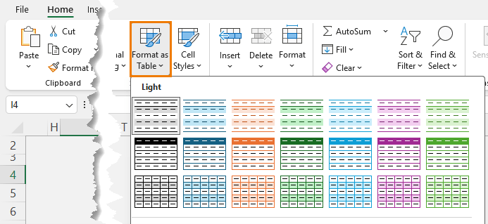
2. Select it and go to Home > Format as Table.
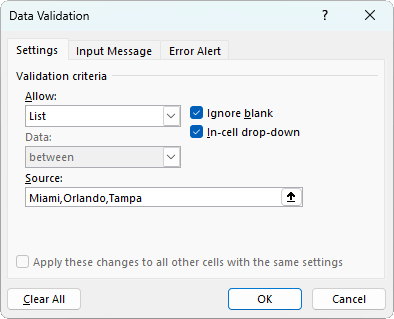
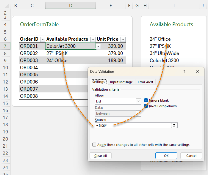
3. Create your drop-down list using Data > Data Validation > Allow: List.
4. In the Source box, select the
table column instead of typing values.
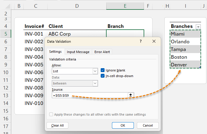
Now, whenever you add new items (e.g., Boston, Denver), your drop-down updates instantly.
⚠️ Note: This method only works if the list is on the same sheet. Let’s fix that next.
2. Lists on Other Sheets with Named Ranges
When your lists live on a separate worksheet (for tidiness), tables alone won’t auto-update. The solution is named ranges.
Steps:
1. Select your table column and go to
Formulas > Define Name (e.g., DeptList).
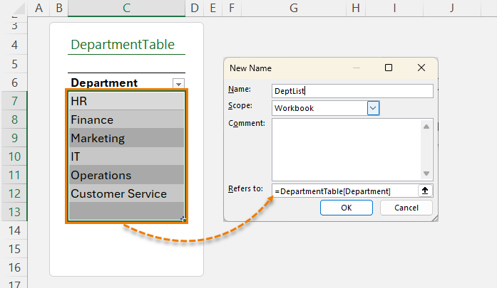
2. In your data validation, reference the name instead of the table column.
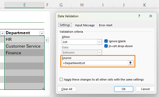
Now all drop-downs in the selected cells automatically include new entries.
💡 Bonus: Combine this with dynamic array formulas like SORT and UNIQUE to clean duplicates and blanks:
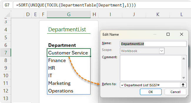
=SORT(UNIQUE(TOCOL(DepartmentTable[Department],1)))
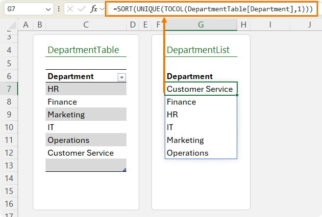
Define a name for this spilled list (e.g., DepartmentList) and reference it in your drop-down.
3. Dependent (Cascading) Drop-Downs
Want a list that changes depending on another selection? For example:
- In the Product Category column select Electronics → see only laptops, tablets, and monitors.
- Or select Furniture → see only desks, chairs, and cabinets.
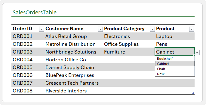
This is a dependent (or cascading) drop-down list.
How to set it up:
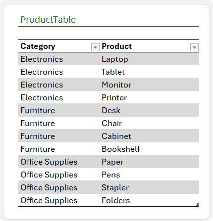
1. Build a lookup table of categories and products.
2. Use the SORT and FILTER functions to spill the product lists based on
the category in row 6:
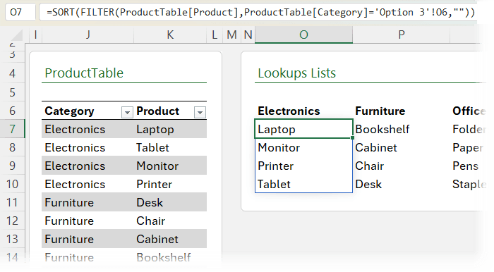
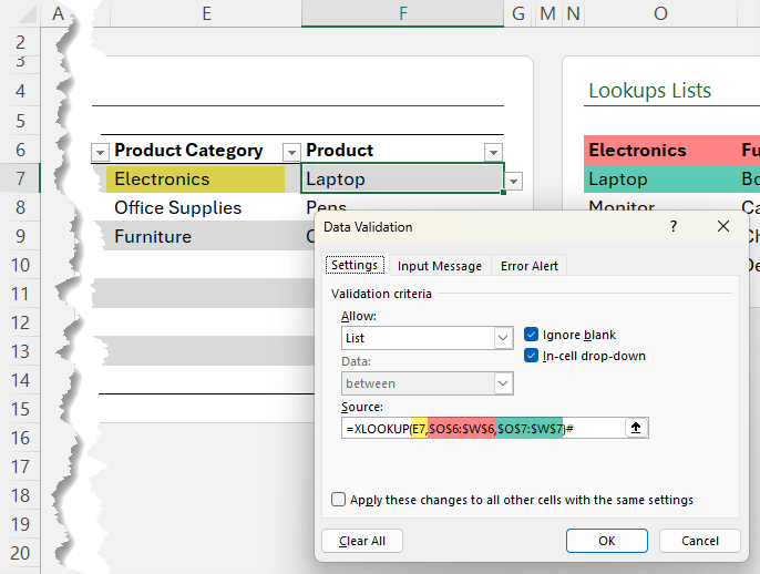
3. Use XLOOKUP to reference these spilled ranges in your data validation.
Result: error-proof data entry, faster selection, and a much cleaner experience.
Note: Check
out the video above for step-by-step on setting up the lookup table so that it automatically updates as you add more product categories and products.
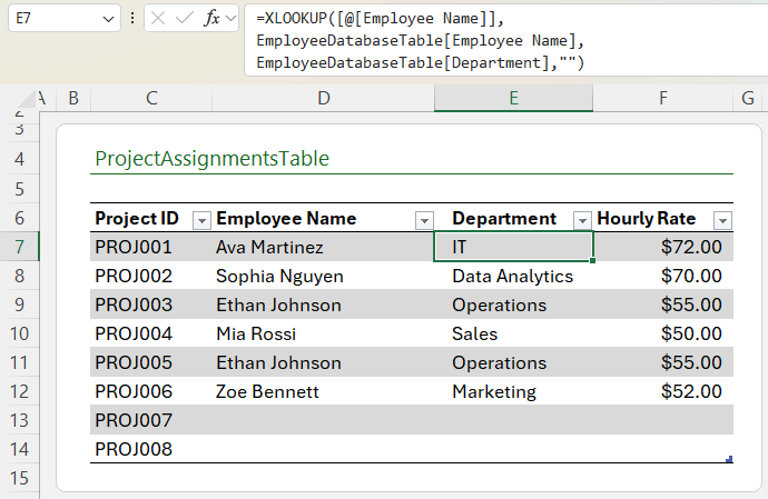
4. Drop-Downs That Fill in Related
Data
Drop-downs can do more than limit choices, they can also auto-populate related information.
Example: Choose an employee in a drop-down, and Excel automatically fills in their Department and Hourly
Rate.
Formula:
=XLOOKUP([@[Employee Name]],
            EmployeeDatabaseTable[Employee Name],
            EmployeeDatabaseTable[Department],"")
Copy across to retrieve multiple fields (e.g., Hourly Rate). This transforms your drop-downs into interactive forms that reduce manual entry and errors.
5. Excluding Items with FILTER
Here’s where modern Excel really shines. Suppose you have a product catalogue with “Active” and “Discontinued” statuses:
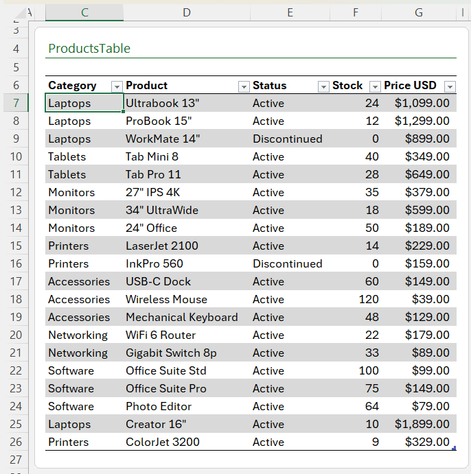
Instead of maintaining two lists, use the
FILTER function.
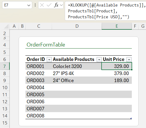
Formula:
=SORT(UNIQUE(FILTER(ProductsTbl[Product],
            ProductsTbl[Status]="Active","")))
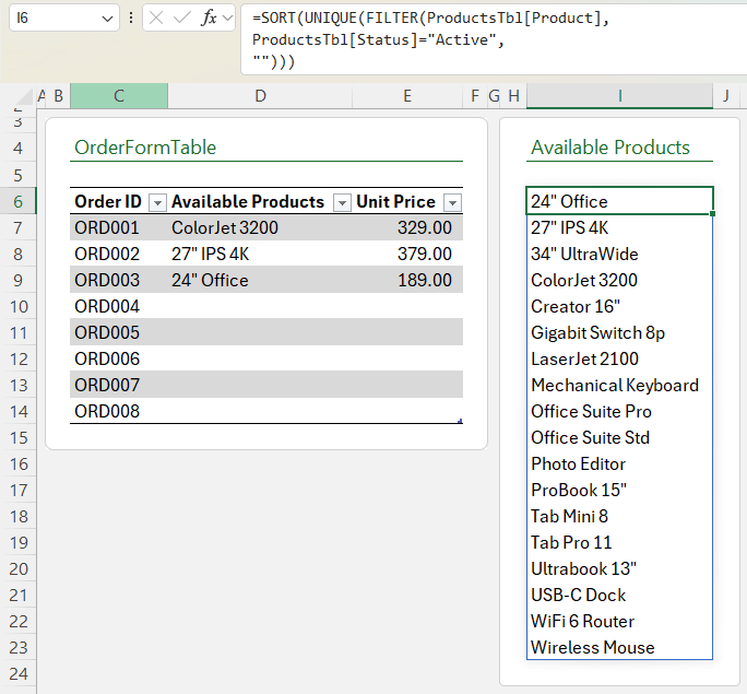
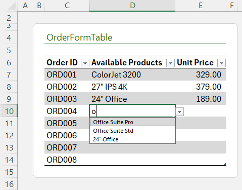
This ensures your drop-down always shows only active products, automatically sorted and de-duplicated:
Pair it with XLOOKUP to return related details (like price).
👉 In newer versions of Excel, drop-downs even let you search as you type, making selection even faster.
Why These Methods Matter
By combining Excel tools like Tables, Data Validation, Named Ranges, and Dynamic Array Functions, you can build drop-downs
that:
- Save time by updating themselves.
- Prevent errors with dependent filtering.
- Provide instant lookup of related data.
- Scale to hundreds or thousands of
options.
This is the difference between “just knowing Excel” and thinking like Excel.
Next Steps
If you want to go beyond drop-downs and master Excel at a professional level, check out my Excel Expert Course. It covers advanced formulas, dynamic arrays and more; complete with real-world projects and my personal mentoring.