1. Asterisk * - The Wildcard for Any Number of Characters
The asterisk is a wildcard used in text-based formulas like COUNTIF or SEARCH. It stands for any number of characters.
Example:
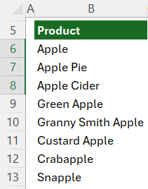
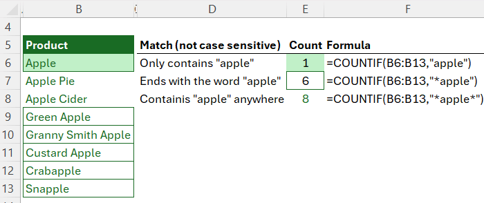
If you want to count how many product names contain “Apple” anywhere in this list:
An asterisk either side of the search term will return all instances of ‘apple’ anywhere in the text string:
=COUNTIF(B6:B13, "*apple*")
=8
Want to find “Apple” only at the end of the text string? Use the asterisk wild card like this:
=COUNTIF(B6:B13, "*apple")
=6
Use it when you need flexible pattern matching in strings.
2. Question Mark ? - The Wildcard for Exactly One Character
The question mark matches exactly one character.
Example:
To sum values for Order IDs that start with “AB12” followed by any one character from this list:
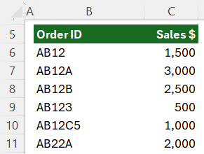
Use the question mark in SUMIF like this:
=SUMIF(B6:B11, "AB12?", C6:C11)
=$6,000
Want to allow two characters after “AB12”? Just use two question marks:
=SUMIF(B6:B11, "AB12??", C6:C11)
=$1,000
Use ? when the pattern has a fixed number of varying characters.
3. Tilde ~ - Escape Character for
Wildcards
What if you want to find an actual * or ? in your data?
Use the tilde ~ before the symbol to treat it as a literal character.
Example:
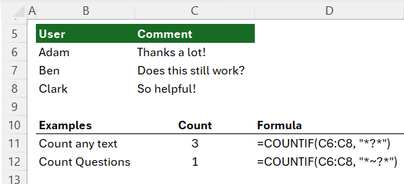
=COUNTIF(C6:C8, "*~?*")
This counts cells that literally contain a question mark anywhere in the text string.
On row 12 of the screenshot below you can see the difference between
using the tilde to count text containing instances of a question mark surrounded by any number of characters vs the formula on row 11 which counts all cells because *?* is essentially saying count any cell that contains at least 1 character.
Use tilde to escape special characters:
~? → search for a real question mark
~* →
search for an asterisk
~~ → search for the tilde itself
4. Curly Braces {} - Define Arrays
Curly braces are used to define arrays directly in formulas.
For example, let’s say you want to create a series of quarter starts dates for 2025.
We can use the DATE function:
Syntax:
=DATE(year, month, day)
And instead of a single month number, we can use an array of the months we want returned:
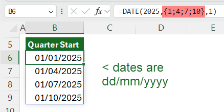
This returns a vertical array but if you want a horizontal array, replace the semicolons separating the month numbers in the array with commas:
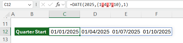
Excel 2019 and Microsoft 365 automatically spill the results. In older versions of Excel, you’ll need to select the cells you want the dates returned to first, then press Ctrl + Shift + Enter to complete the formula.
5. Trim Ref Dot Operator . - Trim Empty Cells in Ranges
This new feature lets you dynamically trim ranges by using a dot before or after the colon range operator. It ensures Excel only refers to cells containing data while allowing new data to be included automatically, resulting in more efficient calculations.
Example:
=SUM(C6:.C20)
This tells Excel to ignore any trailing empty cells at the bottom. You can also trim from the top with a dot
before the colon:
=SUM(C6.:C20)
or both with a dot either side of the colon:
= SUM(C6.:.C20).
For even more flexibility, try the new TRIMRANGE function, which trims rows and columns together.
6. Hash # - Refer to Spilled Arrays
If you're using dynamic arrays like UNIQUE, the # symbol lets
you refer to the entire spilled range.
Example:
In the screenshot below you can see cells F7:F10 contain a UNIQUE formula that spills an array of 4 values. As shown in cells I6:J6, I can count those values with COUNTA by simply referring to
the first cell in the spilled array followed by a hash sign:
=COUNTA(F7#)
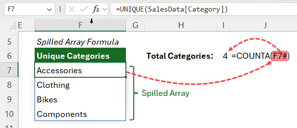
This spilled array references adjusts automatically as new data spills into the array, so I never need to update my COUNTA formula.
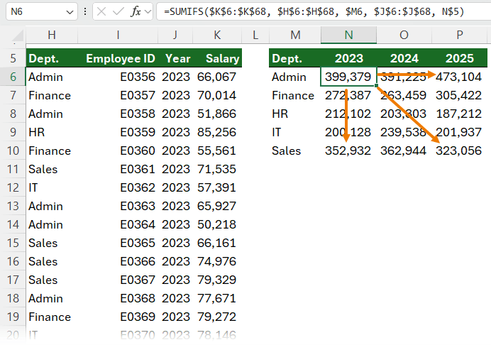
7. Dollar Sign $ - Lock References
The $ symbol locks parts of a reference in place when copying formulas.
Examples:
- $A$1 - Absolute row and column
- A$1 - Absolute row only
- $A1 - Absolute column only
Use the F4 key to quickly toggle between these when writing or editing formulas.
The SUMIFS formula below illustrates the use of mixing relative and absolute references which enables the formula to be written once for cell N6 and then copied to the remaining cells in the table:
8. Square Brackets [ ] - Structured References in Tables
When working with Excel Tables, column references use square brackets:
Example:
Find the sum of the Stock column in the Table below (the Table name is ‘Stock’):
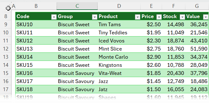
We can use the SUM function and reference the table name and column name inside square brackets:
=SUM(Stock[Stock])
Likewise, for the total of the
Value column:
=SUM(Stock[Value])
Tip: You can type the structured references in or select the table column with your mouse and have Excel complete it for you.
Note: Structured references don't respond to F4. You must use extra brackets to lock them. More on making Excel Table Structured References absolute here.
9. At Symbol @ - Current Row in Tables
Inside Excel Tables, the @ symbol refers to the current row. The formula in column G below multiplies the values from the current row’s Price and Stock columns:
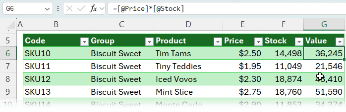
This formula is exactly the same on every row and because it’s inside a table, it will automatically copy it down the column and apply it to any new rows added to the
table.
Outside the table, you need to include the table name:
=Stock[@Price]*Stock[@Stock]
IMPORTANT: the @ symbol only works
if the formula is in the same row as the data it's referencing.
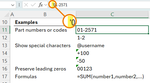
10. Apostrophe ' - Force Text Format
Starting a cell with an apostrophe tells Excel to treat the entry as text — even if it looks like a number, formula, or date.
Examples:
- '01-2571 — Stops Excel converting it into a date
- '00123 — Keeps leading zeros
- '=$A$1+B1 — Displays the formula without calculating it
The apostrophe is invisible in the cell, but you’ll see it in the formula bar.
Conclusion: Use Symbols Intentionally
Symbols like *, @, { }, #, and [ ] may seem minor, but they pack a punch. Understanding how Excel interprets them gives you greater control over your formulas and spreadsheet design.
If you're ready to level up even further, check out our Advanced Excel course — built for professionals who want to build smarter, faster, and more reliable spreadsheets.