Outdated Excel Functions – Step-by-step
1. VLOOKUP / HLOOKUP → XLOOKUP
The VLOOKUP function has long been a go-to lookup tool, but it has serious limitations — it only looks right, it breaks when you insert columns, and it returns approximate matches unless you specify otherwise.
Better Alternative: XLOOKUP
Syntax: =XLOOKUP(lookup_value, lookup_array,
return_array, [if_not_found], [match_mode], [search_mode])
Feature | XLOOKUP | VLOOKUP / HLOOKUP |
Search direction | Any direction (left, right, up, down) | Top to bottom (VLOOKUP) or left to right (HLOOKUP) only |
Lookup column/row position | Lookup can be in any column or row | Must be
first column (VLOOKUP) or first row (HLOOKUP) |
Exact match by default | ✅ Yes (default is exact match) | ❌ No (default is approximate which is error prone) |
Approximate match | ✅ Yes (optional) | ✅Yes (default) |
Return multiple columns / rows | ✅ Yes (can return multiple columns/rows
easily) | ❌ No (one value only) |
Insert/delete column or row
issues | ✅Doesn't break because lookup and return arrays are separate | ❌ Breaks if columns/rows are inserted or
deleted |
Error handling (custom messages) | ✅Built-in with the
optional [if_not_found] argument | ❌ Need to wrap with IFERROR manually |
Support for dynamic arrays (spilled arrays) | ✅Yes | ❌ No |
Search from first or last match | ✅ Yes (search_mode option) | ❌ No |
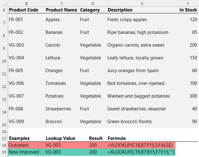
Taking the data below, you can see the comparative formulas on rows 18 and 19:
Check out the deep dive XLOOKUP function tutorial.
2. CONCATENATE / CONCAT → TEXTJOIN
Combining text from multiple cells used to require clunky formulas — and blank cells would result in unwanted double spaces or missing separators.
Better Alternative: TEXTJOIN
Syntax: =TEXTJOIN(delimiter, ignore_empty, text1,...)
Feature | TEXTJOIN | CONCAT | CONCATENATE |
Skip blanks | ✅ Yes (ignore_empty) | ❌ No | ❌
No |
Separator support | ✅ Built-in | ❌ No | ❌ No |
Combine ranges directly | ✅ Yes | ✅ Yes | ❌ No (must list each cell) |
Supports
array formulas | ✅ Yes | ✅ Yes | ❌ Limited |
Accepts ranges | ✅ Yes | ✅ Yes | ❌ No |
Available in Excel 365 / 2019+ | ✅ Yes | ✅ Yes | ⚠️ Deprecated |
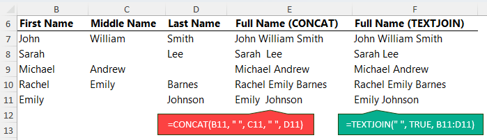
Example: column E below shows the limitation of the CONCAT function when handling empty cells, with a double space between ‘Emily Johnson’ in cell E11, whereas TEXTJOIN in cell F11 handles it with ease:
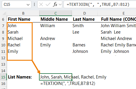
TEXTJOIN can also create lists in a single column and skip any blanks:
For more on the TEXTJOIN function and workarounds for earlier versions of Excel, check out the TEXTJOIN tutorial here.
3. MATCH → XMATCH
MATCH helps find the position of a value in a list - often used with INDEX. But it’s limited
in direction and requires manual match type setup.
Better Alternative: XMATCH
Syntax: =XMATCH(lookup_value, lookup_array, [match_mode], [search_mode])
Feature | XMATCH | MATCH |
Search
direction | Top-to-bottom or bottom-to-top | Only first match (top to bottom) |
Exact match | ✅ Yes (default) | ✅ Yes |
Approximate match | ✅ Yes (simpler
options) | ✅ Yes (needs setting 1 or -1) |
Wildcards support (e.g., * or ?) | ✅ Yes | ✅ Yes |
Find next larger or smaller item | ✅ Yes (easier options) | ✅
Yes |
Return position from bottom | ✅ Yes (search_mode) | ❌ No |
Supports Regex Match | ✅ Yes (native support) | ❌ No |
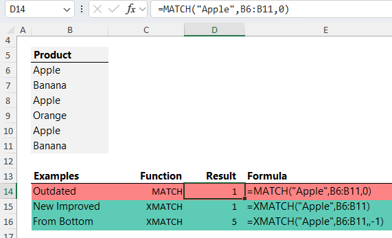
Example: In
the example below, rows 14 and 15 show equivalent formulas. XMATCH doesn’t need the additional match mode argument because an exact match is the default. In row 16 you can see the search from bottom capabilities of XMATCH.
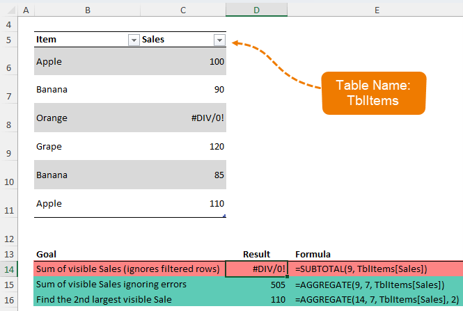
4. SUBTOTAL → AGGREGATE
SUBTOTAL is great for calculating only visible rows, but it falls short when errors are present in the data and has limited aggregation options.
Better Alternative: AGGREGATE
Syntax: =AGGREGATE(function_num, options ref1,...)
Feature | AGGREGATE | SUBTOTAL |
Basic aggregations (SUM, AVERAGE, COUNT, etc.) | ✅ Yes | ✅ Yes |
Option to ignore
nested SUBTOTAL / AGGREGATE results | ✅ Yes | ✅ Yes |
Option to ignore hidden rows | ✅ Yes (with options) | ✅ Yes (function numbers 1–11) |
Option to ignore errors | ✅ Yes | ❌ No |
Supports more functions (e.g., LARGE, SMALL, MEDIAN) | ✅ Yes (19 total functions) | ❌ No (only 11 functions) |
Built-in error handling | ✅ Yes (ignore #DIV/0!, etc.) | ❌ No |
Examples: In the examples below, we can see that while SUBTOTAL fails when there are
errors in the range (row 14), AGGREGATE handles it with ease (row 15). Additionally, AGGREGATE can perform tasks like returning the second largest visible sales value (row 16):
For more innovative solutions, check out the deep dive tutorial on the AGGREGATE function.
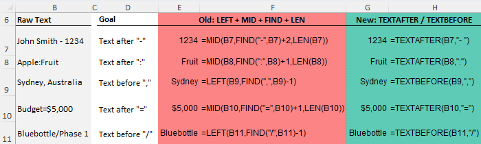
5. LEFT, MID, FIND, LEN → TEXTAFTER, TEXTBEFORE
Extracting parts of text used to require multi-layered formulas that were difficult to build and troubleshoot.
Better Alternative: TEXTAFTER, TEXTBEFORE
Syntax:
=TEXTBEFORE(text,delimiter, [instance_num], [match_mode], [match_end], [if_not_found])
=TEXTAFTER (text,delimiter, [instance_num], [match_mode], [match_end], [if_not_found])
Feature | TEXTAFTER / TEXTBEFORE | LEFT + MID + FIND + LEN |
Syntax complexity | Low (simple and readable) | High (need nested formulas) |
Handles first occurrence easily | ✅ Built-in | ⚠️ Only with careful FIND setup |
Handles second, third, nth occurrence | ✅ Simple (with instance_num argument) | ❌ Hard (needs complex
nesting) |
Easy to extract before / after a delimiter | ✅ Yes
(direct) | ❌ No (manual calculation needed) |
Dynamic delimiter
support | ✅ Built-in | ⚠️ Possible but messy |
Error handling for missing delimiter | ✅ Optional fallback value | ❌ No (Requires IFERROR) |
Examples:
There’s also a sibling function called TEXTSPLIT that enables you to split by multiple delimiters across columns or rows. Check out the
deep dive TEXTBEFORE, TEXTAFTER and TEXTSPLIT tutorial here.
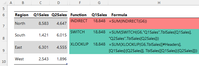
6. INDIRECT → SWITCH or XLOOKUP
INDIRECT was a clever trick to create dynamic references, but it’s volatile and fragile.
Better Alternatives: SWITCH or XLOOKUP
Syntax: =SWITCH(expression, value1, result1, [default_or_value2], [result2],...)
Syntax: =XLOOKUP(lookup_value, lookup_array, return_array, [if_not_found], [match_mode], [search_mode])
Old Use of INDIRECT | Why People Used It | Better Modern Solution |
Dynamic named ranges (e.g. changing the range based on input) | Let users select a range to use (e.g. "Q1Sales", "Q2Sales") | ✅ CHOOSE, XLOOKUP, or SWITCH can now map names directly without needing volatile references |
Selecting columns dynamically | Build a reference like A:A or B:B based on a cell | ✅ Use INDEX(array, , column_number) instead - much faster and non-volatile |
Building dynamic ranges for SUMIFS etc. | Create flexible ranges without manual editing | ✅ Use dynamic arrays (e.g., FILTER, SEQUENCE, INDEX), or structured tables with better
formulas |
Referencing spilled array results indirectly | Point
formulas at spill ranges | ✅ Use # spill references directly now, e.g., =A2# |
Making validation lists
dynamic | Build dropdown lists that grow automatically | ✅ Use dynamic arrays with UNIQUE, SORT, or Excel Tables (structured
references) |
Pulling data from different tables dynamically | Choose which table or range to pull
from | ✅ Use CHOOSE, SWITCH, or structured tables |
Dynamic sheet references (e.g. build a reference like 'Sheet2'!A1) | Needed to reference different sheets based on a cell value | ❌ No true alternative
yet for dynamic sheet names - still need INDIRECT 😕 (or VBA / LAMBDA hacks) |
Examples: Return a dynamic range based on the drop-down list in cell G6 that toggles between the different table (TblSales) columns (C & D):
Check out the deep dive tutorials:
7. OFFSET → Trim Ref Dot Operator or Excel Tables
OFFSET helped create dynamic ranges, but it’s another volatile function that can slow your workbook.
Better Alternatives: Trim Ref Dot Operator or Excel Tables
Feature | OFFSET | Dot Ref | Excel Tables |
Volatile | ✅ Yes | ❌ No | ❌ No |
Dynamic range support | ✅
Yes | ✅ Yes | ✅ Yes |
Spill compatibility | ❌ No | ✅ Yes | ✅ Yes |
Auto-expanding
formulas | ❌ No | ✅ Yes | ✅ Yes |
Trim Ref Dot Operator Example: Column E below contains a dynamic range using OFFSET, compared to column F which uses the trim ref dot operator which is simply a dot after the colon in the first argument C10:.C30:
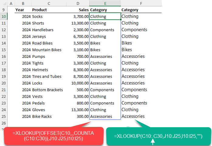
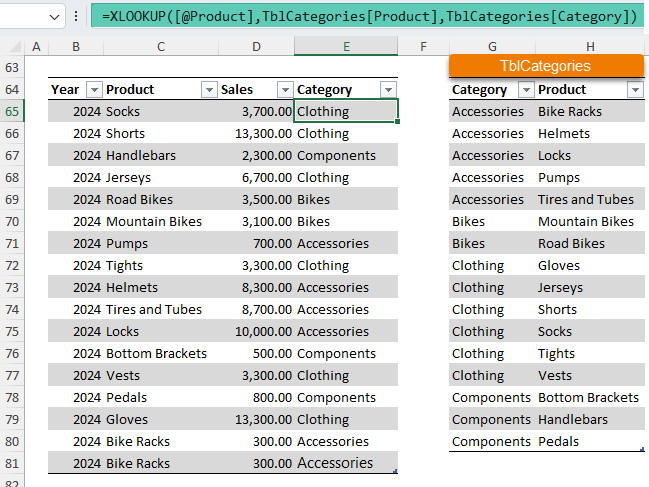
Excel Table Structured Reference Example: In column E, the Category column, the formula uses the table structured references. These automatically include any new data added to the table, without the need for complex formulas like OFFSET:
Note: Dot references work well for formulas that spill arrays; Tables are ideal for structured data and auto-filling.
Check out the deep dive
tutorials:
Want to Go Deeper?
If you'd like help writing cleaner formulas and mastering all the new Excel tools, check out my Advanced Excel Formulas Course. I’ll walk you through step-by-step lessons with examples you’ll actually use at work.