Hi ,

The Excel Bug That Breaks Your Formatting (And How to Fix It) 

Have you ever opened the Conditional Formatting Rules Manager in Excel only to find your rules have mysteriously duplicated or become fragmented? You didn’t create extra rules, so what’s going on?

Don’t worry, this frustrating behaviour has a simple explanation and, better still, a reliable fix. In this post, I’ll walk you through what causes conditional formatting rules to break and two smart solutions to prevent it.

Prefer to read this on our website? 

Then click this link >>> The Excel Bug That Breaks Your Formatting (And How to Fix It)

Video: The Excel Bug That Breaks Your Formatting (And How to Fix It) 

Watch on YouTube

Why Conditional Formatting Rules Duplicate and Fragment

This issue occurs when Conditional Formatting rules use a relative reference to rows above or below the current row.

An example of this is where I used a Conditional Format to create a dynamic merged cell effect. Which, by the way is a great way to have the clean look of merged cells without the limitations.

However, inserting a row into a table or list that uses relative references in its conditional formatting will result in duplicated and fragmented rules which are tedious to tidy up.

Here's what happens:

Suppose your conditional formatting rule is:

=A4=A3

This compares the current cell to the one above it. But if you insert a row, Excel adjusts the reference. And now you have two rules with one that might look like:

=A11=A9

You can see the result in the conditional formatting rules manager below:

That inserted row has caused Excel to fragment your formatting logic; just like how regular formulas behave with relative references.

This duplication and fragmentation isn’t a bug, it’s how Excel handles relative references. But for conditional formatting, it becomes a nightmare to maintain.

Solution 1: Use the OFFSET Function

To stop Excel from adjusting your references, you can use the OFFSET function in your conditional formatting formulas.

Example:

Replace:

=A4=A3

With:

=A4=OFFSET(A4,-1,0) 

Why this works:

• OFFSET(A4,-1,0) returns the value from the cell one row above A4, no matter where the formula is copied.
• All references are anchored to the current row (4), so Excel doesn’t need to adjust anything when rows are inserted or deleted.

But there’s a catch:

OFFSET is a volatile function. If you have a large workbook or many conditional formatting rules, using volatile functions can significantly slow down performance.

Solution 2: Use a Relative Named Range (No Volatile Functions)

If performance is a concern, this clever workaround from Excel expert Neale Blackwood is for you.

Step-by-step:

1. Select a cell, say A4 (you can choose any cell, just not one in row 1 of the workbook).
2. Go to Formulas > Define Name.
3. In the dialog:
   • Name: CellAbove
   • Refers to: =A3 (important: delete all $ signs to make it fully relative)
   • Scope: Set to the current worksheet (unless you plan to use this in other worksheets)

Now, you can use =CellAbove in a formula, and it will always return the value of the cell directly above the current one, no matter where you use it.

Apply it to Conditional Formatting:

Replace:

=A4=A3

With:

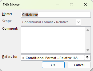
=A4=CellAbove

This method works just like OFFSET, but without any performance penalty. And you can use the same trick to define CellBelow, CellLeft, or CellRight.

OFFSET vs. CellAbove - Which Should You Use?

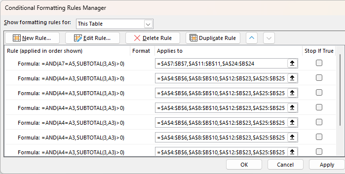
Both solutions prevent your conditional formatting rules from fragmenting:

Try both and see which fits your workflow best.

A Note on Merged Cell Effects with Filtering

If you’re using conditional formatting to simulate merged cells like I did in the Dynamic Merged Cells in Excel post, you might notice a quirk when filtering.

Problem:

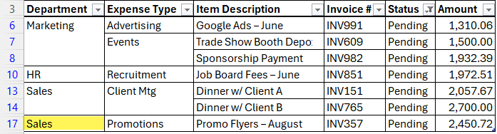
In the image below you can see that when filtering by values like “Pending,” previously hidden department names (e.g., “Sales”) may appear again if rows for other statuses (e.g., “Paid” or “Overdue”) are hidden in between.

Fix:

Use a formula with SUBTOTAL and OFFSET to check visibility and avoid displaying duplicates when filtering.

Example:

=AND(A4=OFFSET(A4,-1,0),SUBTOTAL(103,OFFSET(A4,-1,0)))

This ensures repeated values are only hidden when their preceding row is visible; preventing those odd visual glitches after filtering.

Note: it’s important to only format the border for the top of the cells for this to work. Don’t use ‘all borders’ formatting.

Want More Excel Tricks?

If you’re tired of fixing broken formatting or wondering why formulas aren’t working, my Excel courses teach you how to build spreadsheets that just work. They’re step-by-step, practical, and come with personal support from me.

Have a great day,

Mynda Treacy

Co-founder My Online Training Hub

Want to sponsor our newsletters?  Just reply to this email to get in touch with us.