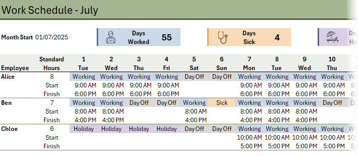
Build a Smarter Work Schedule in Excel (That Updates Automatically)
Watch the video above for step-by-step instructions on how to build an automated work schedule, or follow the written instructions below.
Step 1: Generate the Dates for the Month
1. In
cell B3, enter the start of the month (e.g., 1/7/2025 for 1st July).
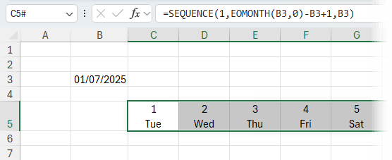
2. In C5, enter the following formula to spill the dates across the row:
=SEQUENCE(1,EOMONTH(B3,0)-B3+1,B3)
3. Format the date cells:
- Select the cells, press CTRL + 1 to open the Format Cells dialog.
- Go to the Number tab → Custom.
- Enter this custom format:
d CTRL+J ddd
(Press CTRL+J between the d and ddd to wrap the day name on a new line.) - Then, go to the Alignment tab:
- Check Wrap
Text
- Set Horizontal Alignment to Center
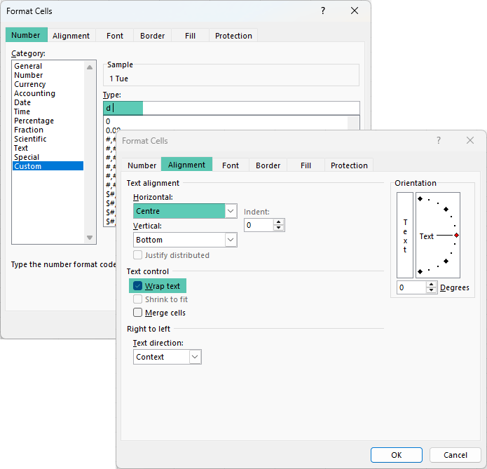
- Increase row height to fit the text.
It should look like this:
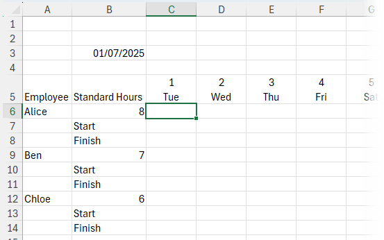
Step 2: Set Up the Employee Table
1. In column A, list your employees:
Example:
- A6: Alice
- A9: Ben
- A12: Chloe
Each employee needs 3 rows:
- Row 1: Work status
- Row 2: Start time
- Row 3: Finish time
2. In column B, input each employee’s standard work hours:
- B6: 8 (Alice)
- B9:
7 (Ben)
- B12: 6 (Chloe)
It should look something like this:
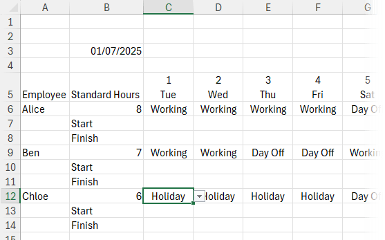
Step 3: Add Drop-Downs for Work Status
1. Select the first row for each employee’s schedule (e.g., C6:AG6 for Alice).
2. Go to Data > Data Validation > List and enter:
Working,Day Off,Sick,Holiday
(Add/remove options from the list to suit your requirements.)
3 .Copy the data validation to each employee’s status row.
4. Set the work status for each employee for the month.
Mine looks like this now:
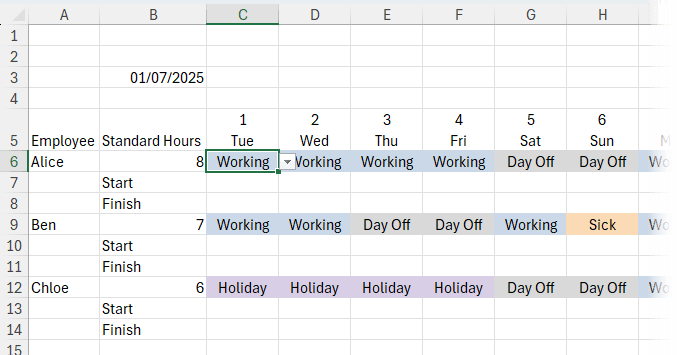
Step 4: Colour-Code Work Statuses
1. Select all status cells (e.g., C6:AG28 to allow space for more employees).
2. Go to Home > Conditional
Formatting > Highlight Cells Rules > Text that Contains.
3. Add rules like:
- “Working” → blue fill
- “Day Off” → grey fill
- “Sick” → orange fill
- “Holiday” → green fill
It’s coming along nicely:
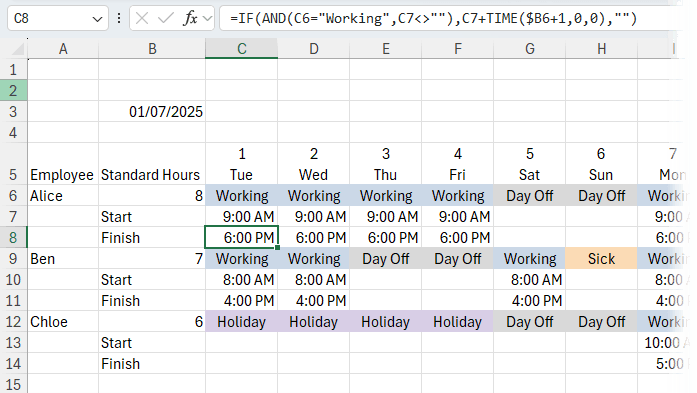
Step 5: Automatically Calculate Finish Times
1. In the second row for each employee, enter their start time (e.g., C7: 9:00 AM).
2. In
the third row (e.g., C8), enter the formula:
=IF(AND(C6="Working",C7<>""), C7+TIME($B6+1,0,0), "")
This checks if the employee is working and has a start time, then adds standard hours +1 hour for lunch. Modify the +1 to suit your
break duration.
3. Copy this formula across the row and down for other employees.
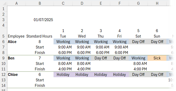
Step 6: Freeze Panes for Easy Scrolling
Select cell C6 > go to View > Freeze Panes > Freeze Panes
Now, names, standard hours and dates in row 5 stay visible while scrolling.
Step 7: Add Visual Dividers Between Employees
1. Select all rows in the schedule (e.g., A6:AG28).
2. Go to Home > Conditional Formatting > New Rule > Use a formula
Use this formula:
=$B6="Finish"
3. Format with a green bottom border to separate each employee’s block.
4. Go to the View tab and turn off gridlines.
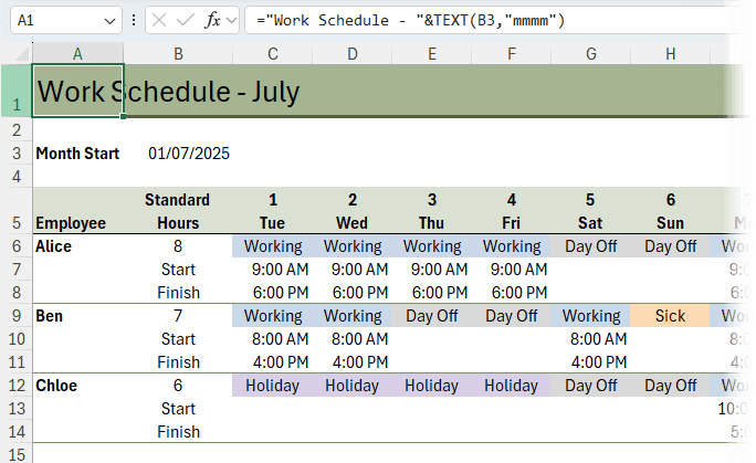
Step 8: Create a Dynamic Heading
1. In cell A1, enter:
="Work Schedule - " & TEXT(B3,"mmmm")
2. Format this row with green fill and white bold text for visibility.
3. While we’re
formatting, let’s also add green fill to row 5 and format the font bold.
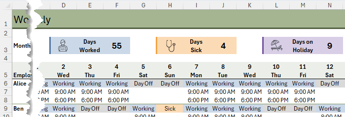
Step 9: Add Summary Figures (Optional but Useful)
1. Use COUNTIF to calculate how many days were worked:
- In E3: label = Days Worked
- In F3:
=COUNTIF(C6:AG30,"Working")
Repeat for “Sick” and “Holiday” if you want more summaries.
2. Add icons using Insert > Icons, search for:
- Computer (working)
- Doctor
(sick)
- Sun (holiday)
Resize and colour to match your theme.
Step 10: Customize and Expand
- To add new employees, just insert a new 3-row block and copy formatting and formulas.
- You can change the standard hours, start times, or status drop-downs to suit your team.
Next Steps
If you enjoy this kind of logic-based setup and want to feel more confident using formulas like these, I teach everything from Excel formulas to dashboards and Power Query in my online Excel courses here,
These are the exact tools I rely on when building templates like this, and they’ll help you go from basic spreadsheets to time-saving systems.