Hi ,

Dynamic Merged Cells in Excel 

At first glance, (regular) merged cells can make your spreadsheet look clean and polished - just the way most teams like it. But beneath that tidy surface, they wreak havoc on your ability to filter, sort, analyse, and summarize data.

In this guide, I’ll show you why merged cells break Excel functionality - and exactly how to create dynamic merged cells in Excel without compromising on readability or layout.

Prefer to read this on our website? 

Then click this link >>> Dynamic Merged Cells in Excel

Video: Dynamic Merged Cells in Excel

Watch on YouTube

Why Merged Cells Are a Problem for Filters & PivotTables

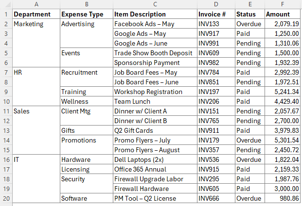
Let’s say you’ve got a table with merged cells in the “Department” and “Expense Type” columns. It looks great—until you try to:

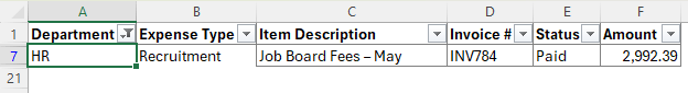
• Filter the data: Filtering by a column like “Department” for the HR transactions won’t return all matching results because merged cells break row alignment:

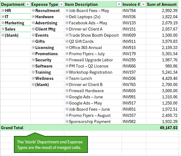
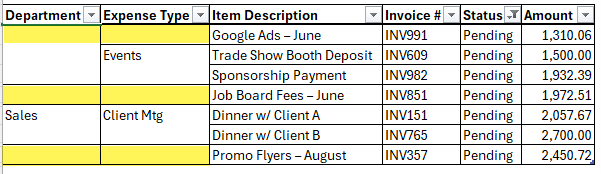
• Build PivotTables: Only the first row of each group retains the department name; the rest are counted as blanks:

• Sort your data: Sorting is a non-starter with Excel refusing to play nice when merged cells aren’t the same size:

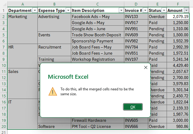
• Use formulas: Referencing merged cells in formulas becomes unreliable and painful.

Bottom line: Merged cells might look good, but they break Excel’s core features.

The Better Way: Dynamic Merged Cells = Clean Layout + Full Functionality

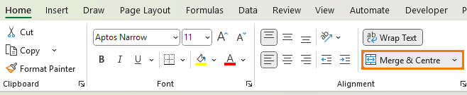
Step 1: Unmerge the Problem Cells

• Select the “Department” and “Expense Type” columns.
• Go to Home > click Merge & Center to unmerge them.

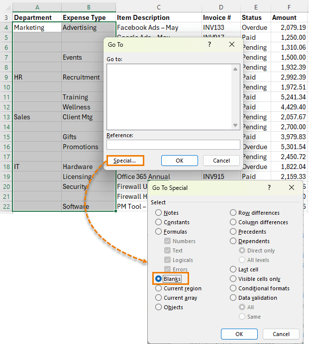
Step 2: Fill the Empty Cells

To restore the data structure:

1. Select the columns again.

2. Press Ctrl+G > Special > choose Blanks.

3. With the blanks selected, type = and press the Up Arrow key.

4. Press Ctrl+Enter to apply the formula to all selected cells.

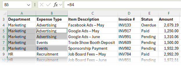
5. Copy the columns, then Paste Special > Values to remove the formulas.

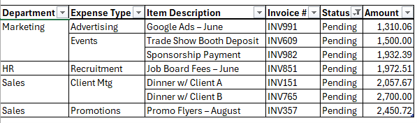
Now every cell contains the correct label, and your dataset is clean and functional.

Step 3: Turn It Into a Smart Excel Table

• Select a single cell in your dataset or the whole table and press Ctrl+T to create a table.
• Select a clean, white style (e.g., “White Table Style Light 15”) and turn off banded rows if preferred.
•  

Tip: Excel Tables also make your data easier to manage, analyze, and reference in formulas.

Step 4: Visually Clean It Up with Conditional Formatting

Now your data works—but it’s cluttered with repeated values. Let’s hide them (visually only) using Conditional Formatting formulas.

Hide Repeats with a Custom Format

1. Select the “Department” and “Expense Type” columns (excluding the headers).
2. Go to Home > Conditional Formatting > New Rule.
3. Choose “Use a formula to determine which cells to format.”
4. Enter the formula:
   =A4=A3
   (Adjust for column as needed, and use relative references by pressing F4 three times.)
5. Click Format > Number > Custom, and enter this format code:
   ;;;
   (This hides the content but retains full functionality.)
6. In the Borders tab, remove the Top Border so repeated values visually merge with the ones above.

This makes your table much easier to scan, without using actual merged cells.

Step 5: Fix Filtering Issues

When you filter the table, the conditional formatting still compares hidden rows, which can cause the first visible row of a group to appear blank as you can see in the screenshot below.

Solve it with the AGGREGATE Function

With the AGGREGATE function we can check if the row above is visible:

=AGGREGATE(3,5,A3)

• 3 counts non-empty cells.
• 5 tells Excel to ignore hidden rows.
• A3 refers to the cell above the current row.

Combine it with your existing rule:

=AND(A3=A2, AGGREGATE(3,5,A2))

Apply this formula in your Conditional Formatting rule to ensure that hidden rows don’t affect the visibility logic.

Now when you filter by “Pending” or any other criteria, only the appropriate values are hidden, making everything work as intended:

One Caution: Inserting or Deleting Rows

Conditional Formatting rules that reference relative rows (like A3=A2) can break when you insert or delete rows. Excel will fragment/duplicate the rule in the background.

There’s a more advanced workaround using the OFFSET function let me know in the comments if you want a full breakdown of that approach!

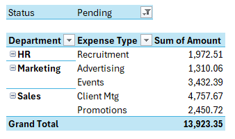
The Payoff: Flawless PivotTables and Clean Analysis

With your table now properly structured:

• Insert a PivotTable via Insert > PivotTable.
• Add Department to Rows and Amount to Values.
• Add Status to Filters and choose “Pending”.

Now you’ve got a professional breakdown of your data that updates dynamically - without a single merged cell in sight:

Wrap-Up: Clean Layouts Without Sacrificing Functionality

Merged cells might look neat, but they cause more problems than they solve. By unmerging, filling blanks, and using Conditional Formatting tricks, you create dynamic merged cells that keep your spreadsheet clean and functional.

Want to Take It Further?

Check out my Excel Expert Course if you want to master layouts, formulas, PivotTables, and analysis workflows.

Have a great day,

Mynda Treacy

Co-founder My Online Training Hub

Want to sponsor our newsletters?  Just reply to this email to get in touch with us.