The Problem with Copying Excel Table Formulas
Let’s say you’re using a formula like this:
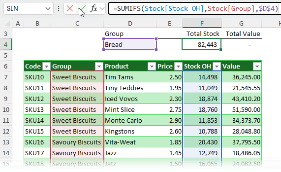
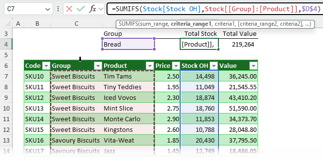
=SUMIFS(Stock[Stock OH], Stock[Group], $D$4)
This sums the “Stock OH” column based on a “Group” match in D4 as shown below:
Sounds great… until you copy it.
- Copy/paste (Ctrl+C, Ctrl+V): Structured references are treated as absolute. That means they don’t shift when pasted - great if that’s what you want, but usually it’s not.
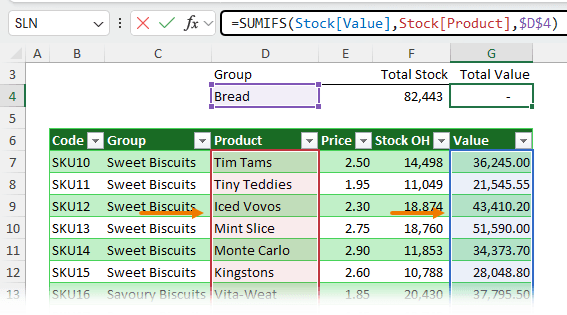
- Left-click and drag: Structured references are treated as relative. When you drag the formula across, the column references shift - and your formula breaks:
So, how do you lock a specific table reference?
Locking a Single Column
Reference in a Table
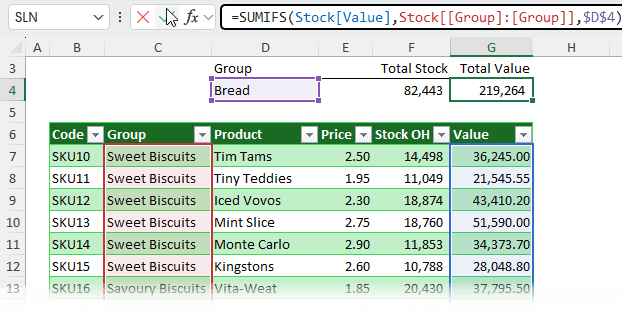
To lock a column like Stock[Group], wrap it in an extra set of square brackets and repeat the column reference like this:
Stock[ [Group] : [Group] ]
Note: Spaces added for clarity.
This tells Excel: lock the reference from the Group column to the Group column - essentially, just this column.
Now when you drag the formula across, it won’t shift.
Shortcut to Insert Table Structured References Quickly
Instead of manually
typing double brackets and colons, select two columns in the formula editor. For example:
Stock[[Group]:[Product]]
as shown below:
Then just replace ‘Product’ with ‘Group’ and you're done. Excel writes the double brackets and colon etc. for you, plus no memorizing syntax required.
Locking
Multiple Columns in Table References
Double brackets work for ranges too:
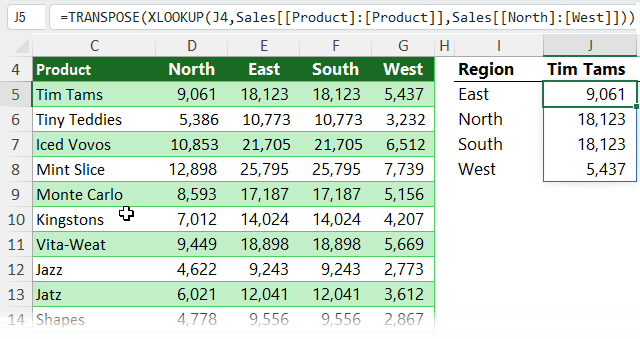
=XLOOKUP(J4, Sales[[Product]:[Product]], Sales[[East]:[West]])
- The first part looks for a match in the Product column
(locked).
- The second part returns values from East to West (locked by default when multiple columns are selected with your mouse).
To return these horizontally but spill vertically, wrap it in TRANSPOSE (see screenshot below):
=TRANSPOSE(XLOOKUP(J4, Sales[[Product]:[Product]], Sales[[East]:[West]]))
Making
Multi-Column References Relative
By default, Excel locks multi-column references like:
=SUM(Sales[[North]:[East]])
Copy it across and it won’t shift.
To make it relative, remove the double brackets and prefix each column with the table name.
=SUM(Sales[North]:Sales[East])
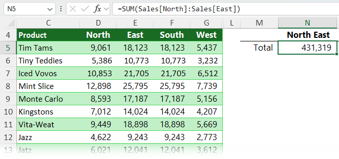
Now it will shift when copied across - perfect for side-by-side calculations.
Locking Row References in Excel Tables
When working inside a table, Excel uses the @ symbol to refer to values in the current row:
= [@Allocation] * [@[Admin Overhead]]
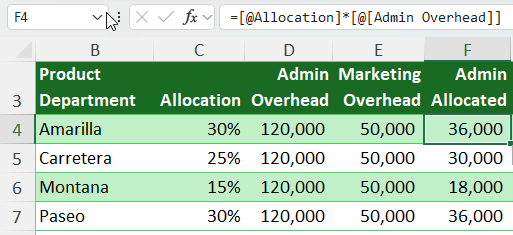
Drag it across and - uh oh - it shifts columns.
To lock it:
1. Select a multicell range across columns like cells C4:D4, Excel will insert the structured reference with the double brackets and colon already inserted:
=Overheads[@[Allocation]:[Admin Overhead]]
2. Then replace
the second column with the actual one you want and complete your formula:
= Overheads[@[Allocation]:[Allocation]] * [@[Admin Overhead]]
Now it's locked.
Referencing Rows in a
Table
You can also reference multiple columns in the same row:
=SUM(Overheads[@[Admin Allocated]:[Marketing Allocated]])
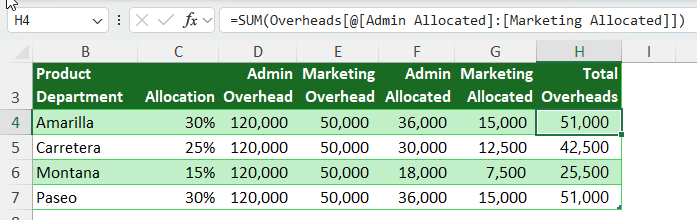
This sums across columns in the same row.
Tip: If the column name has
no spaces (like Allocation), you can even skip the extra brackets after the @ sign:
=[@Allocation]
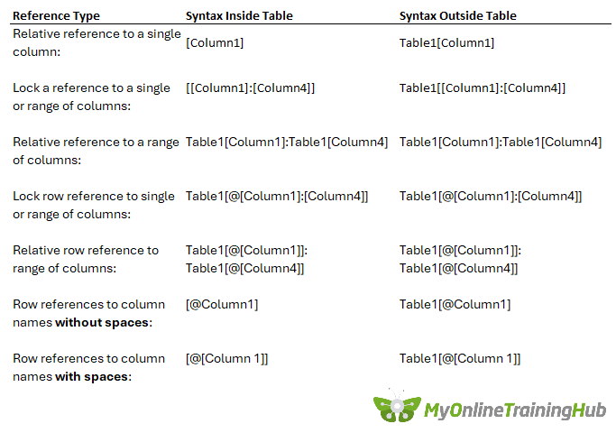
Cheat Sheet: Table Reference Syntax
I know there’s a lot of scenarios, so I included this cheat sheet in the Excel file you can download above to help you quickly find what you need:
Tip: Don’t try to memorize
these - just use the mouse and have Excel insert them for you, then tweak as needed.
Final Thoughts
Locking structured references isn’t always intuitive, but once you know the double bracket trick and the mouse shortcut to insert them, it becomes second nature. Whether you’re locking rows, columns, or ranges, the key is using the right syntax for the right copy method.
Are you using Excel Tables to their full potential? See what else Tables can do, check out our comprehensive Excel Tables lesson here.