Hi ,

These Excel Functions Make Data Analysis Easy

Over a billion people use Excel and let's guesstimate half of them know how to write an IF formula.

Of that 500 million, 99% don't fully understanding how Excel handles logical tests.

This knowledge can be the difference between writing monstrous nested IF formulas like this one below that contains 15 IFs, and 5 CEILING functions:

=CEILING(IF(C11="consignment ",(IF($G11>30,(CEILING(IF($B11="Station A",IF($F11>10,($B$4-$D11+$F11),($B$4-$D11)),IF($F11>10,($B$5-$D11+$F11),($B$5-$D11))),10)+(H11-AGO/365*30*IntRate)),(CEILING(IF($B11="Station A",IF($F11>10,($B$4-$D11+$F11),($B$4-$D11)),IF($F11>10,($B$5-$D11+$F11),($B$5-$D11))),10)))+20),(IF($G11>30,(CEILING(IF($B11="Station
A",IF($F11>10,($B$4-$D11+$F11),($B$4-$D11)),IF($F11>10,($B$5-$D11+$F11),($B$5-$D11))),10)+(H11-AGO/365*30*IntRate)),(CEILING(IF($B11="Station A",IF($F11>10,($B$4-$D11+$F11),($B$4-$D11)),IF($F11>10,($B$5-$D11+$F11),($B$5-$D11))),10))))),10)/FXRate

And this formula that returns the same result without using IF at all:

=CEILING( XLOOKUP(B11,$A$4:$A$5,$B$4:$B$5,,0)-D11+(C11="Consignment")*20+(F11>10)*F11+(G11>30)*(H11- AGO/365*30*IntRate),10)/FXRate

But more than that, understanding how Excel handles logical tests is fundamental to many areas of Excel like advanced filters, conditional formatting and more.

Prefer to read this on our website? 

Then click this link >>> Excel Logical Functions

Video: These Excel Functions Make Data Analysis Easy

Watch on YouTube

.

Let's look at the common logic functions like AND, OR, NOT and XOR that you might think are easy, but I'll show you their limitations and the alternatives.

Plus, I'll show you why you don't need to even use IF a lot of the time and what to do instead, which can vastly improve your formulas.

Lastly, I'll show you under the hood of how Excel uses logic in arrays, enabling you to perform calculations you can't do with the built-in logic functions.

Along the way I'll drop some tips and tricks that will take your Excel skills to pro level.

How Excel Handles Logic

The logic functions, AND, OR, NOT and XOR all return a single TRUE or FALSE result. These are Boolean values and in Excel they are a data type all their own.

Boolean logic is a form of algebra where all values are reduced to either TRUE or FALSE. In Excel, TRUE can also be represented with 1 and FALSE with 0.

AND Function

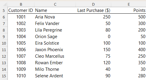
Let’s say you’re hosting an exclusive preview of your new product line for your most loyal customers. Invitations will be sent to those who have spent $100 or more. and have 300 or more points.

In column F of the table below I've used the AND function to find which customers qualify for an invitation:

The AND function takes a series of logical tests and returns TRUE where all tests are TRUE, and FALSE where any test is FALSE.

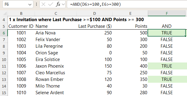
The limitation is I want it to return a number so that I can add up how many invitations I need to issue.

I can do this with the double unary, which is simply two minus signs. The double unary coerces the TRUE and FALSE values into their numeric equivalents of 1 and 0 like so:

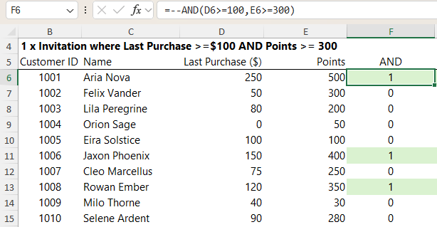
And now I can easily add them up. Another way I can add them up without coercing them first, is inside the SUM function like so:

=SUM(--F6:F15)

However, I don't even need to use the AND function. I can simply write the logical tests inside parentheses and multiply them by one another:

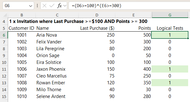
Notice here I haven't used the double unary, and this is because performing a math operation on Boolean values also coerces them into their numeric equivalents.

Best Formula: At this point you're probably wondering which is best and the answer is, whichever you prefer.

In this scenario there's no clear winner, but there are some limitations to the AND function that you don't get with the pure logical tests.

Limitations: With all these solutions I still need to calculate the logical tests one row at a time before I can add them up to find out how many invitations I'm sending out.

In this scenario it makes sense to do so because I need to identify which customers to send invitations to vs just finding out how many to print.  But that's not always the case and I'll share a solution to this later.

Takeaways:

• The double unary coerces TRUE and FALSE values into their numeric equivalents,
• as do math operations.
• Multiplying logical tests is the same as using the AND function.

OR Function

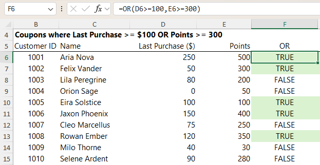
Your next promotion is to send a discount coupon to individuals who either have spent more than $100 OR have over 300 points (or both).

Below I've used the OR function to handle the logical test and return the results.

The OR function takes a series of logical tests and returns TRUE where one or more tests are TRUE, and FALSE where all tests are FALSE.

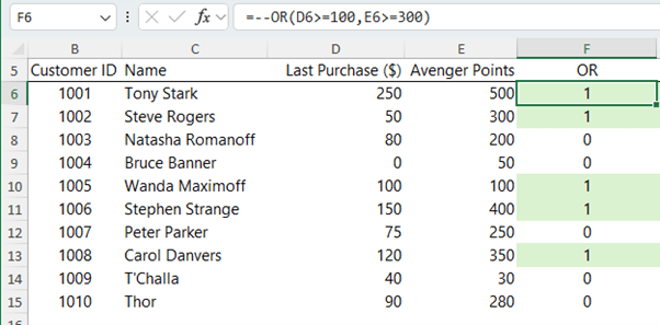
Again, I can coerce the Boolean TRUE and FALSE values to their numeric equivalents with the double unary:

And I can write it without using OR by adding the logical tests like so:

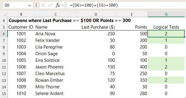
However, notice that when both logical tests are TRUE the result is 2 because TRUE+TRUE is the same as 1+1.

In some cases this might be the desired result. 

However, here I only want to give the customers who met either criterion, one briefing. It wouldn't make sense to send out the briefing twice.

A solution to this is to wrap the logical tests in the SIGN function. SIGN converts positive values to 1, zeros to 0 and negative values to -1.

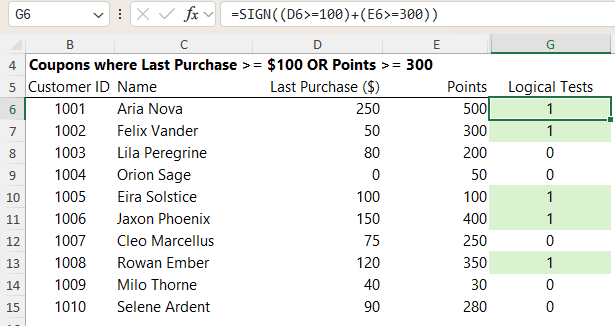
Best Formula: In this scenario there's no benefit to using the SIGN function over the OR function, but later we'll see where SIGN may be useful.

Takeaways:

• Adding logical tests treats them as OR criteria.
• The SIGN function can be used to convert results to 1 where more than one logical test is TRUE.

NOT Function

Next, we’ll target customers who have NOT made a purchase yet with a special introductory offer to encourage their first purchase.

We can identify customers who haven't made a purchase using the NOT function:

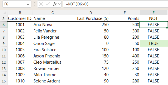
Of course, we can also write this with a simple logical test like so:

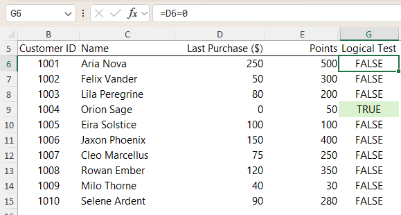
Let's say we wanted to identify customers who had made a purchase. It could be written with NOT like so:

=NOT(D6=0)

Or as a logical test:

=D6<>0

Best Formula: Personally, I find the double negative in a NOT function more difficult to write than the simple logical test above.

XOR Function

The XOR function stands for ‘Exclusive Or' and returns TRUE when the number of TRUE inputs is odd and FALSE when the number of TRUE inputs is even.

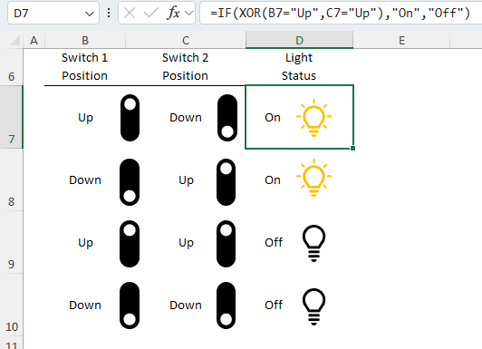
The easiest way to think of XOR is with the light switch scenario. Let's say we have two light switches that control the same light, one at each end of a hall or staircase. The light is only on when the two switches are in different positions.

In the table below, where the light status is TRUE, the light is on, and FALSE it's off:

For our next promotion we’ll invite customers who have either spent less than $100 or have less than 200 points, but not both, to a preview event for a new product.

We could write it like so:

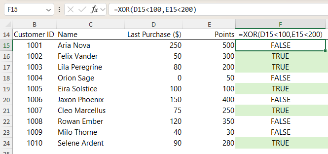
It could also be written with logical tests nested in ISODD:

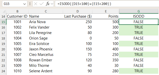
Best Formula: In this scenario I'd guess that XOR might be more efficient to calculate that the pure logical tests inside ISODD, but it probably wouldn't be noticeable on less than 100k rows of data.

If, however you want to return an array of Boolean values, then ISODD is the winner because XOR can only return a single result. More on returning arrays in a moment.

IF Alternative

This time we want to give each customer who has not made a purchase a super bonus of 2 Invitations to our next product launch, so they can bring a plus 1.

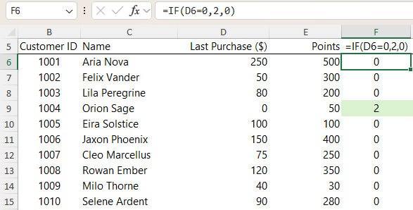
However, when we require a numeric result from a logical test, the IF function is often redundant.

In this case I could simplify this formula like so:

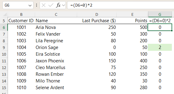
No double unary is required because I'm multiplying the result of the logical test by 2, which coerces it into its numeric equivalent.

Best Formula: There's no standout winner here, but I'd hazard a guess that the pure logical test will be slightly faster for Excel to calculate, but not significantly on small datasets.

Takeaways: IF is often not required when the outcome of the formula is numeric.

Nested IF/IFS Alternative

Nested IFs or the newer IFS function enable you to perform a logical test, return a result if the test is TRUE, if not, it will move on to the next logical test and so on until it finds a TRUE outcome.

In this scenario we want to reward customers with a coupon worth 20% of their last purchase where they spent >$200 or 10% of their last purchase where they spend >$100.

We can write this with a Nested IF or the newer IFS function:

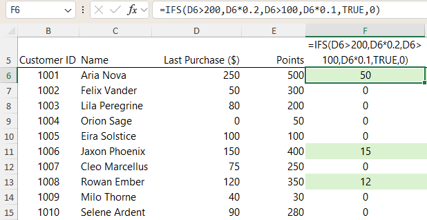
Or with the older nested IFs like so:

=IF(D6>200,D6*0.2,IF(D6>100,D6*0.1,0))

Or we could simplify it with pure logical tests:

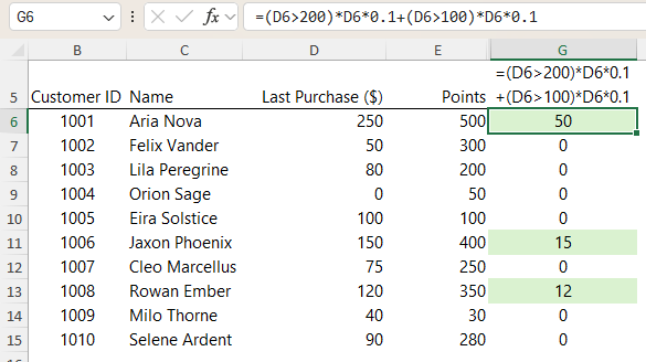
Note here that both logical tests are performed, hence why both only calculate 10% of the coupon value. Because once combined, customers who spent >$200 will receive 20% in total.

Best Formula: The nested IF formula will be more efficient for Excel to calculate because they stop calculating at the first logical test that returns TRUE, whereas the pure logical test formula and IFS formula will always calculate all logical tests.

Takeaway: IFS and Nested IF formulas stop calculating at the first logical test to return TRUE. This means it's crucial to get the order of logical tests correct. For more on this, check out my comprehensive tutorial on IF, Nested IF and IFS formulas.

Arrays

OR, AND, XOR and NOT can only return a single value. i.e., they can't spill results or return arrays of Boolean values when nested inside other functions.

Therefore, when using functions like FILTER, SUM and SUMPRODUCT among others, that can take an array of Boolean TRUE and FALSE values (or their numeric equivalents of 1 and 0), we need to use the pure logical tests with * for AND, and + for OR.

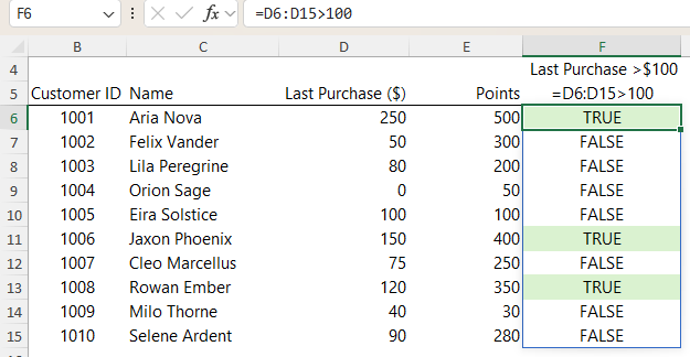
Scenario 1: Let’s say we want to know how many customers spent >$100.

In the image below notice the range being referenced contains all the sales (D6:D15), which are then tested to see if they're > 100. The resulting formula spills the results i.e., it returns an array of Boolean values:

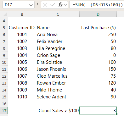
I can also do this in a single cell. The double unary shown in the image below coerces the TRUE and FALSE results from the logical test to their numeric equivalents of 1 and 0 for SUM to add up.

Scenario 2: Lets find the value of purchases where customers spent more than $100 OR have more than 200 Points.

With pure logical tests I can reference the whole range of purchases (D6:D15) and Points (E6:E15) and perform the logical test on the array, which returns arrays of results.

Remember, with OR criteria I must wrap the logical tests in the SIGN function where there's a possibility of double counting.

Here I'm performing my logical tests on different columns, which means there is a risk that both criteria could be TRUE which would result in double counting.

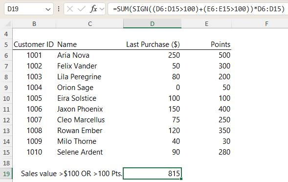
The formula above evaluates like so. The logical tests are evaluated to return arrays of Boolean results:

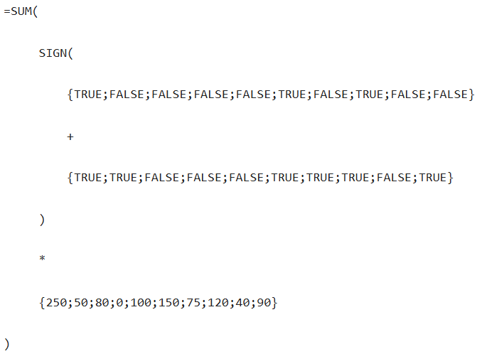
The arrays of Boolean values are then added together:

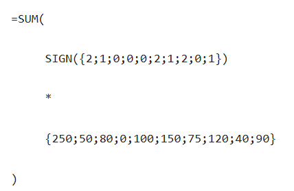
SIGN then converts the positive values to 1 and zeros remain as is:

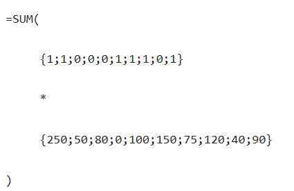
The two arrays are then multiplied by one another to leave an array of values for SUM to add up:

=SUM({250;50;0;0;0;150;75;120;0;90})

=735

Scenario 3: We want a list of customers whose last purchase is >$100 OR that have more than 200 Points. I can use the FILTER function for this which is available in Excel 2021 onward.

The FILTER function references the array (cell range) you want filtered, you then provide it with logical tests that tell it which rows you want returned.

It has 3 arguments, the last being optional, which I won't use in this example:

=FILTER(array, logical tests specifying which rows to include, [if empty])

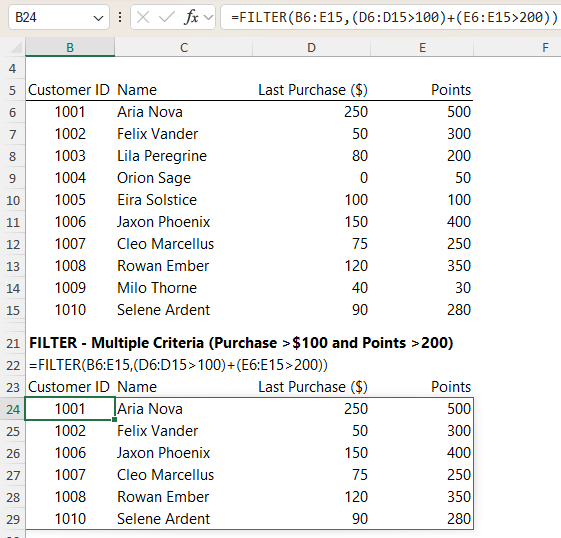
Twist: notice I haven't wrapped the logical tests in the SIGN function! This is because all I need to provide FILTER with are Boolean TRUE and FALSE values or their numeric equivalents.

I'm performing a math operation on my two logical tests which will convert them to their numeric equivalents of 1 and 0, and when added together it evaluates to this:

=FILTER(B6:E15,{2;1;0;0;0;2;1;2;0;1})

And here's the thing 99.9% of Excel users don't realise:

Excel will treat any positive or negative number as TRUE where it requires a Boolean value.

With FILTER there's no risk of it returning a row twice, it simply wants to know if a row should be included or not. Therefore, I don't need to use the SIGN function to convert the array to 1s and 0s.

Bonus Tip: this also applies anywhere Excel operates on Boolean values, including Conditional Formatting rules.

This is just the tip of the iceberg when it comes to FILTER. 

It's one of my favourite new functions in Excel and now that you have logic in Excel mastered, you're ready to maximise the use of FILTER do some amazing things. Go ahead and learn FILTER next:

Excel Filter Function Comprehensive Tutorial including Hacks

Next Steps

When you understand the fundamentals of Excel functions and formulas it enables you to work more creatively and efficiently.

Build on what you've learned here in my Advanced Excel Formulas course and start standing out from the crowd with skills that will get you noticed and promoted.

Have a great day,

Mynda Treacy

Co-founder My Online Training Hub

Want to sponsor our newsletters?  Just reply to this email to get in touch with us.