1. Formula Order of Evaluation
In Excel, understanding the order of operations is key, especially for calculations like Profit %, calculated as:
Note: Above formula calculates Profit %, to calculate Profit Margin, simply use Selling Price in the
denominator.
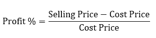
Question 1: Insert a formula in cells E7:E11 to calculate the Profit % for the data below:
Answer 1: In cell E7, the formula is:
=(D7-C7)/C7
Remember, Excel
prioritizes division over subtraction, so wrapping (D7-C7) in parentheses ensures correct calculation. Small details like these often trip up users, so mastering this can set you apart.
To remember the order, use the PEMDAS acronym:
Parentheses,
Exponents,
Multiplication and
Division, and
Addition and
Subtraction
2. Counting Functions
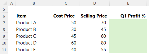
Excel's counting functions are powerful tools for data analysis. Using this data:
Answer the following questions using the correct Excel function:
Question 2.1 - How many employees do we have age data for?
Answer 2.1: - COUNT: Counts numeric values in a range:
=COUNT(C5:C14)
Returns 6 employees with age data.
Question 2.2 - How many employees are listed in the table?
Answer 2.2 - COUNTA: Counts both numbers and
text:
=COUNTA(B5:B14)
Counts all employees listed, returning 10.
Question 2.3 - How many email addresses are missing?
Answer 2.3 - COUNTBLANK: Counts blank cells in a range, useful for identifying missing information like email addresses:
=COUNTBLANK(D5:D14)
Returns 4 employees without email
addresses.
Question 2.4 - How many employees are aged over 30?
Answer 2.4 - COUNTIF: Counts cells meeting a specific condition:
=COUNTIF(C5:C14,">30")
Returns 3 employees over age 30.
Learning Resources:
3. Logical Functions
Logic functions, such as IF and AND, are excellent for
creating conditional formulas. Using the data below:
Answer
the following questions:
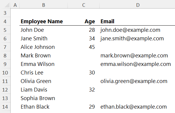
Question 3.1 - Write a formula to determine if the "Monthly Sales" for each employee have reached a sales target of 5000 or more. If they have, return "Met"; otherwise, return "Not Met."
Answer 3.1 - Simple IF Statement: To check if an employee's monthly sales have met a target (e.g., $5,000), use:
=IF(E12>=$G$9,"Met","Not Met")
Question 3.2 - Write a formula that checks if the "Monthly Sales" are greater than 8000 and the
"Performance Score" is 4 or higher. If both conditions are true, calculate a bonus of 5% of Sales, otherwise return 0.
Answer 3.2 - IF with AND Condition: For more complex conditions, such as calculating a 5% bonus if sales exceed $8,000 and performance is 4 or higher, use:
=IF(AND(E12>$H$9, F12>=$H$10),E12*0.05,0)
Learning Resources:
4.
Lookup Functions
Every Excel user needs proficiency in lookup functions. Referencing this lookup table:
Answer the questions below to populate columns F and G in the table below:
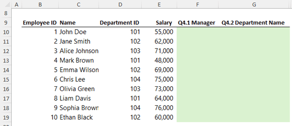
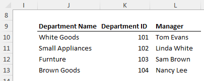
Question 4.1 - In column F, lookup the department ID in column K and return the Manager Name.
Answer 4.1 - VLOOKUP: To find a manager's name by department ID, use:
=VLOOKUP(D10,$K$10:$L$13,2,0)
Question 4.2 - In column G, lookup the department ID in column K and return the Department Name. Bonus points: return the results as a spilled array.
Answer 4.2 - XLOOKUP (Excel 365): This flexible function handles multiple conditions and spilled arrays:
=XLOOKUP(D10:D19,K10:K13,J10:J13)
Learning Resources:
5. Text Functions
Text manipulation often requires creative formulas. Using the data below:
Answer the following questions.
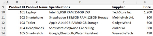
Question 5.1 - In column G write a formula to combine the product name and price formatted with $, comma separators and 2 decimal places. e.g. Laptop - $1,200.00
Answer 5.1 - Combining Text: To combine a product name and its formatted price, use:
=C10&" - "&TEXT(F10,"$#,###.00")
Question 5.2 - In column H, write a formula to split the specifications out into their separate components as delimited by the semi-colon.
Answer 5.2 - Splitting Text: In Excel 365, use TEXTSPLIT to separate data by a specific delimiter. For
instance,
=TEXTSPLIT(D10,";")
Splits specifications listed with semicolons. For older Excel versions, Text to Columns offers a manual alternative.
Learning Resources:
6. PivotTables
PivotTables allow for rapid data summaries. Using the data below:
Answer the following questions.
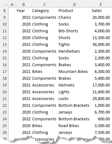
Question 6.1 - Insert a PivotTable in cell G8 that summarises the Sales in the table below by Category down the rows.
Bonus Points: reference the data in a way that allows new data and updates to automatically be included upon refresh.
Answer 6.1:
- Convert your data to an Excel Table (CTRL+T) to enable automatic updates.
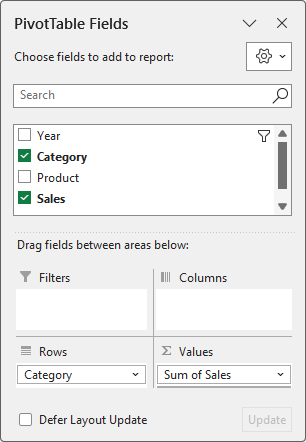
- Insert a PivotTable (Insert tab) to summarize sales by category. The field list should look like this:
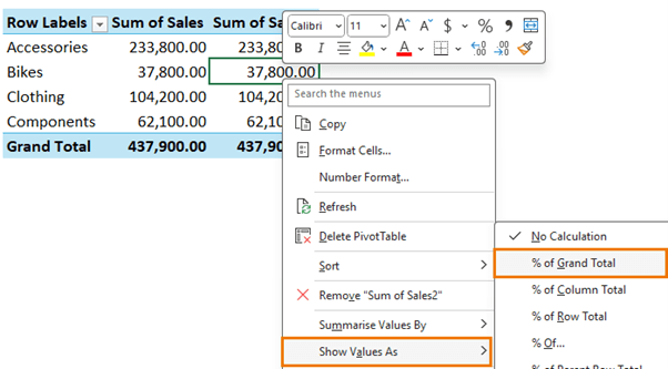
Question 6.2 - Add a column to the PivotTable that calculates the percentage each category's
sales are of the total.
Answer 6.2 - To calculate each category's sales percentage, add the sales field twice to the Values area, right click > Show Values As > % of Grand Total.
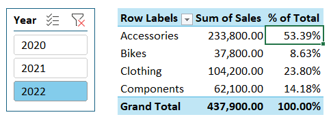
Question 6.3 - Filter the PivotTable for the year 2022 using a Slicer.
Answer 6.3 – Right-click the Year field in the PivotTable field list > Insert Slicer
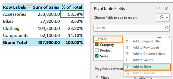
Select the year 2022 in the Slicer
Learning Resources:
7. Data Cleaning
Cleaning data
is crucial in Excel. The next question looks at a common data cleaning task and assesses if the candidate is familiar with a useful shortcut for filling empty cells using the data below:
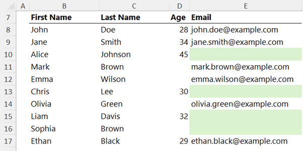
Question 7 - Fill the empty email address cells with a formula that creates the email address from the [email protected] |
Bonus Points: Select all the empty cells before typing in the formula and then enter the formula in all selected cells in one go. |
Answer 7 - Select all blank cells in the column using the Go To Special tool: (CTRL+G > Special > Blanks).
Enter the following formula:
=LOWER(B10&"."&C10&"@example.com")
And press CTRL+ENTER to apply it across all selected blanks.
8. Advanced Skills: Combining Multiple Techniques
For this final task, we'll combine several Excel skills to identify and filter duplicate entries in the data below:
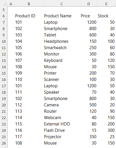
Question 8.1 - Identify the duplicate rows in the dataset.
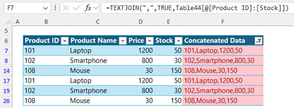
Answer 8.1 part 1 - Format your data as a table (CTRL+T), then add a column that concatenates the row data using TEXTJOIN or CONCAT.
=TEXTJOIN(",",TRUE,Table44[@[Product ID]:[Stock]])Or:
=CONCAT(Table44[@[Product ID]:[Stock]])
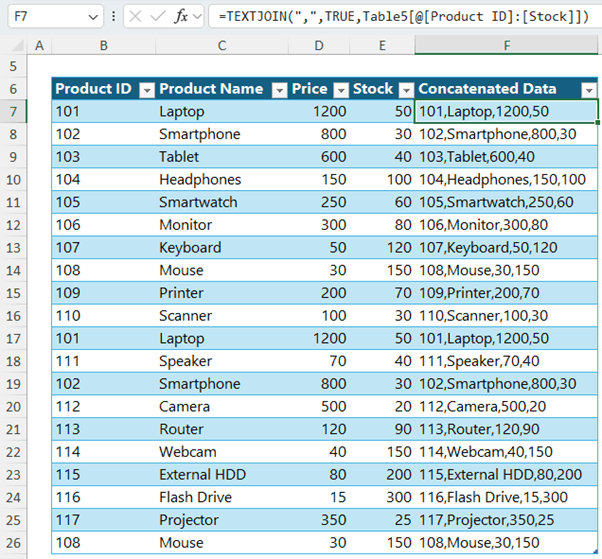
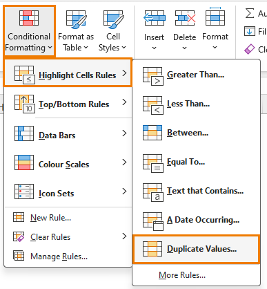
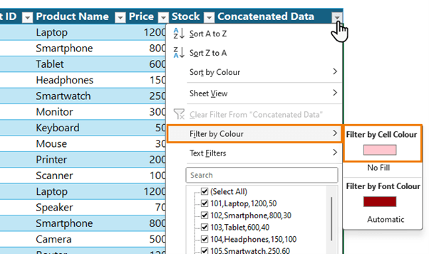
Answer 8.1 part 2 - Conditional Formatting. Home tab > Conditional Formatting > Highlight Cells Rules > Duplicate Values
Question 8.2 - Filter the dataset to only show duplicate rows.
Answer 8.2 - Filter by Colour: Filter the table to display only duplicate entries by filtering based on
cell colour.
Returns the table filtered for
duplicate rows only:
Learning Resources:
Excel Tips for
Interview Success
Level Up Your Skills
As you've probably noticed, knowing your way around Excel functions is crucial. That's exactly why I created a course focused on mastering Advanced Excel formulas.
Each topic is covered in short, easy-to-follow videos, and you'll get practice questions to solidify your skills plus support and mentoring from me personally
Keep Abreast of New Features
Excel's continuous evolution means that staying updated on new features and functions can give you an edge.
For example, learn about Excel's latest tools in our video on Excel's new TRIMRANGE and trim reference
operator that changes the way Excel cell references are written.
And make sure to keep honing your skills to impress in your next interview!