Why Power Pivot?
Traditional PivotTables allow you to summarize and analyze data effectively, but when it comes to larger datasets or more complex calculations, they can fall short.
Power Pivot is an advanced tool built right into Excel, designed to handle these more demanding
tasks.
Here's what makes Power Pivot a game-changer:
- Multiple Data Sources: Integrate data from various sources, such as Excel tables, databases, online services and more.
- Advanced Calculations: Use powerful formulas and data analysis expressions (DAX) for complex calculations using a function language that's modelled on Excel's.
- Speed and Performance: Work with millions of rows of data without slowing down Excel.
Now let's dive into the details of how to use Power
Pivot in your everyday workflow.
Enabling Power Pivot in Excel
Before using Power Pivot, you need to ensure it's enabled in your version of Excel. Here's how to do it:
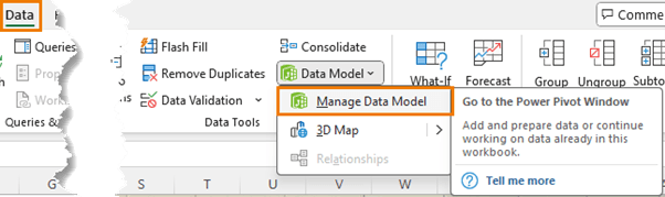
1. Check for Power Pivot in the Ribbon: Go to the Data tab and
look for the Data Model button. If you see it, great! You're ready to go.
2. Activate Power Pivot: If Power Pivot is missing, follow these steps:
- Go to the File tab > Options.
- Choose Add-Ins from the sidebar.
- In the Manage dropdown, select COM Add-ins and click Go.
- Check the box next to Microsoft Power Pivot for Excel and click OK.
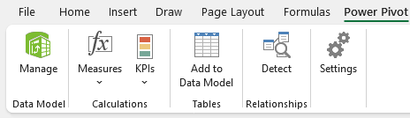
Once activated, Power Pivot will appear as a new tab in your ribbon:
Loading Data into Power Pivot
Now that Power Pivot is ready to use, let's load some data. For this example, we'll work with a movie dataset, spanning 1976 to 2016, which includes fields like director ID, budget, popularity, and revenue.
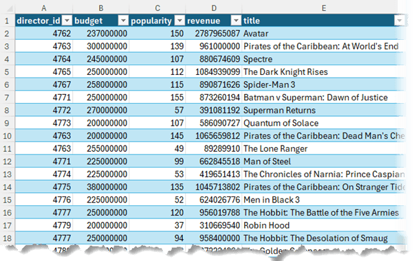
The movie data is in an Excel
Table named 'Movies'.
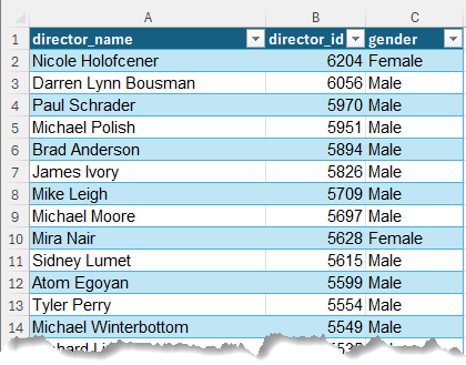
There is also a table with the directors' names and gender in an Excel table named 'Directors':
Steps to Load Data:
- Select the First Table: Click any cell in your first table.
- Add to Data Model: In the Power Pivot tab,
click Add to Data Model.
- Repeat for Other Tables: Do the same for additional tables (e.g., the Directors table).
By loading these tables into Power Pivot, you bypass the need for complex lookup functions like VLOOKUP or XLOOKUP, reducing formula clutter and keeping your file size down.
Connecting the Tables: Creating
Relationships
The magic of Power Pivot happens when you start linking tables using common fields. For example, let's connect our Movies and Directors tables using the director_id field they share.
- Open Diagram View: In the Power Pivot window, switch to Diagram View to visualize the relationships between
tables.
- Drag and Drop: Simply drag director_id from one table to the other, creating a relationship between them.
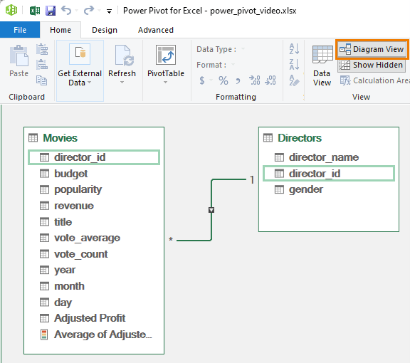
Power Pivot automatically detects a one-to-many relationship, where each director in the Directors table only appears once, but they can have multiple movies associated with them in the Movies table.
This ability to
connect tables allows you to analyze data across multiple tables in one report, without the need for extra formulas.
Creating a Power Pivot PivotTable
With your data loaded and linked, it's time to build a PivotTable that pulls from both tables:
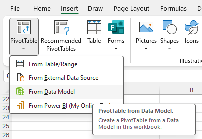
1. Create the PivotTable: From the Power Pivot window, go to the Home tab and click PivotTable. Alternatively, from the Excel ribbon, go to Insert > PivotTable > From Data Model.
2. Choose Fields: In the field list, you'll now see fields from all tables. Add director_name to the rows and revenue to the values to summarize total revenue by director.
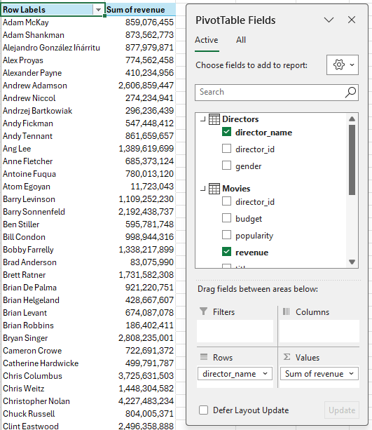
You've now built a report that spans multiple tables, showcasing revenue by director name.
Advanced Techniques: Calculated Columns and KPIs
Now that you've got a basic report, let's take it up a notch by adding calculated columns and Key Performance Indicators (KPIs).
Creating a Calculated Column:
- Open Power Pivot Window
- Add a New Column: Scroll to the right until you see an empty column labelled Add Column, select
it.
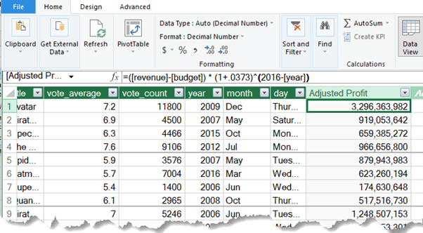
- Enter a Formula: In the formula bar, type =[revenue] - [budget] to calculate the profit for each movie. Press Enter and rename the column to Profit.
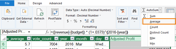
- Adjust for Inflation: For a more accurate analysis, adjust for inflation with the formula:
=([revenue] - [budget]) * (1 + .0373) ^
(2016 - [year])
This gives you an adjusted profit figure that accounts for inflation over time.
Setting Up KPIs:
1. Create a Measure: In the Power Pivot window, select the Profit column and choose Average from the AutoSum dropdown. This creates a measure that will be used as the baseline for the KPI.
2. Define Thresholds: Right-click the measure and select Create
KPI.
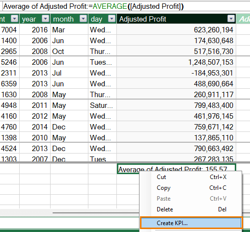
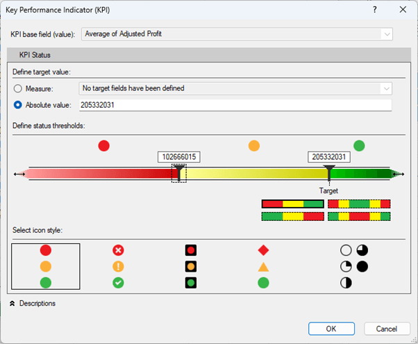
3. Set your
thresholds—reference another measure, or set absolute values — and customize the colors and icons.
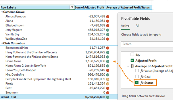
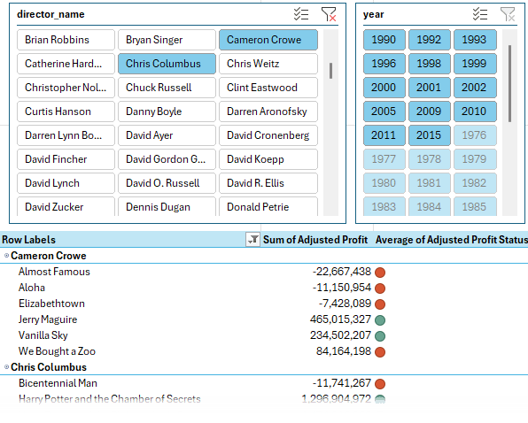
4. Visualize in a PivotTable: Add this KPI to your PivotTable to track how each director's movies perform against the average profit.
Making Your Report Interactive with Slicers
Finally, to make your PivotTable more interactive, let's add Slicers:
1. Insert a Slicer: Select a cell in the PivotTable and go to Insert > Slicer. Choose director_name to easily filter the report by director.
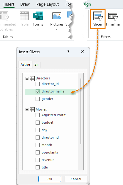
2. Multiple Slicers: You can add more Slicers for fields like year and gender, giving you dynamic control over the data.
Next Steps
Power Pivot is a robust tool that allows you to supercharge your data analysis in Excel. Whether you're dealing with large datasets, multiple data
sources, or complex calculations, Power Pivot provides the flexibility and power you need.
To take your skills further, consider diving into our Power Pivot & DAX course—the ultimate guide to mastering
this tool and transitioning to Power BI effortlessly.
Curious about how to streamline your data loading process with Power Query? Check out our next tutorial for automating boring data gathering and cleaning tasks with Power
Query.