5 Essential Excel Spreadsheet Automation Tricks
1. Auto-Expanding Data Validation
Scenario: Classifying data/data entry - let's say one of the monthly tasks required to update your reports is to classify bank transactions into sub-categories. To ensure
consistency, a data validation drop-down list is set up for choosing sub-categories:
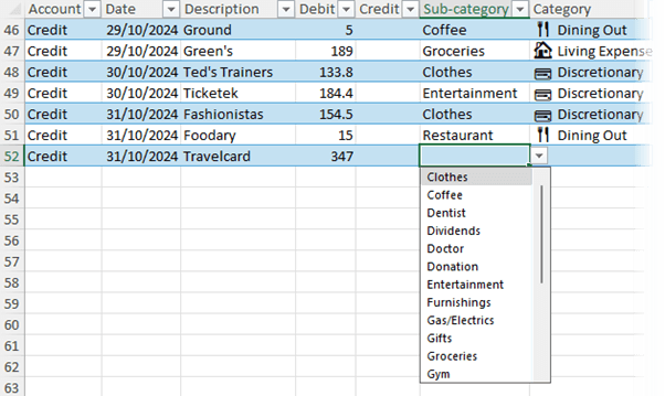
However, new sub-categories may be needed over time. Here's how to make your data validation lists automatically include new
items:
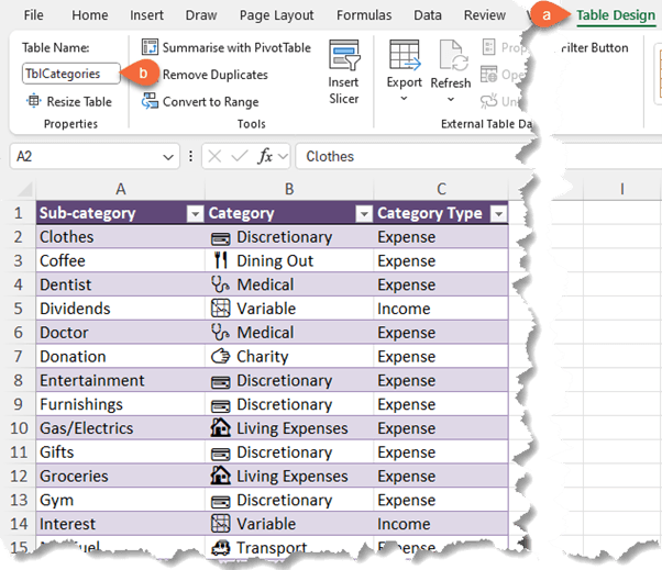
1.1 Format Data in a Table
Place your sub-categories list in an Excel Table via the Insert tab > Table or the shortcut CTRL+T. On the Table Design tab (a), give the table a more useful name (b).
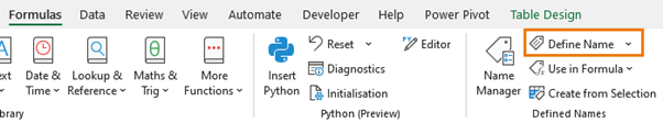
1.2 Define a Name for Sub-Categories
Select the sub-categories
column in the table (excluding the header) and on the Formulas tab > Define Name:
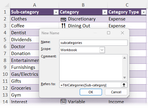
Enter the name 'subcategories' in the New Name dialog box:
1.3 Use Defined Name in Data
Validation
Go to the Transactions table, select the sub-category column, and set the data validation list source to the defined name.
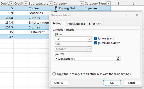
Any new sub-categories added to the Categories table will automatically appear in the drop-down list without any extra effort.
2. Importing Data with Power
Query
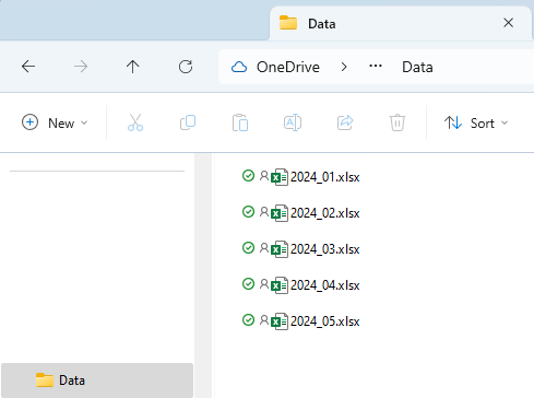
If your report update process involves new data from CSV, text, or Excel files, you can automate the data consolidation with Power Query. For example, below I have 5 Excel files that I need to extract the data from and place in a
single table for my report:
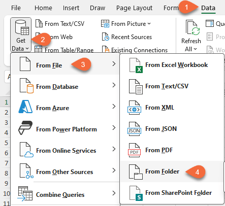
2.1 Get Data from Folder
On the Data tab > Get Data > From File > From Folder.
Select the folder containing your files.
2.2 Combine & Transform Data
Combine the files into a single table.
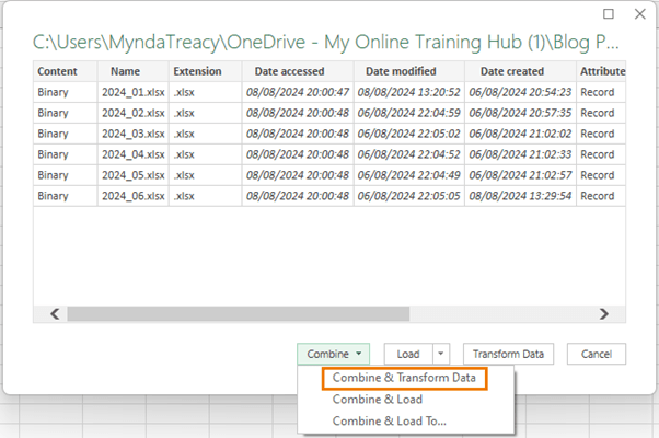
Use the query editor to clean and transform data as needed, such as removing duplicates or adding calculated
columns. See video for step-by-step instructions.
2.3 Load Data
On the Power Query Editor Home tab > Close & Load To…:
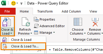
Choose to load the data to a Table, PivotTable, or Pivot Chart.
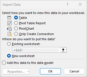
Tip: Loading directly to a PivotTable or Pivot Chart is more efficient and keeps
the file size smaller.
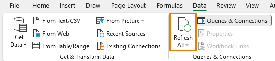
2.4 Update Data
When next month's data is available, simply add the file to the folder and on the Data tab of the ribbon, Refresh All to update your tables, PivotTables, and charts.
3. Structured References
Excel Tables' structured references automatically expand and contract
to include new data. This feature eliminates the need to edit cell references in formulas, PivotTables, or charts:
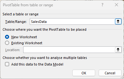
3.1 Insert PivotTables and Pivot Charts
Use the table data to insert a PivotTable and chart. Notice the table name automatically appears in the Table Range field:
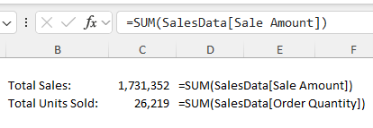
3.2 Reference Table in Formulas
Use the Table's structured references in formulas to ensure they automatically pick up any changes in the table
size:
3.3 Update Data
When new data
is added, refresh the table and all associated formulas, PivotTables, and charts will update automatically.
4. Dynamic Named Ranges
If you can't use tables for some reason, dynamic named ranges are a great alternative. They grow and contract with your data just like structured references for Tables.
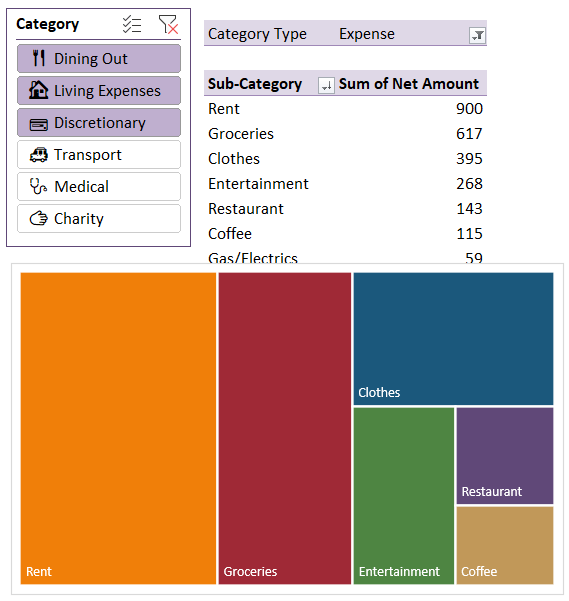
For example, some charts like the treemap aren't compatible with PivotTables:
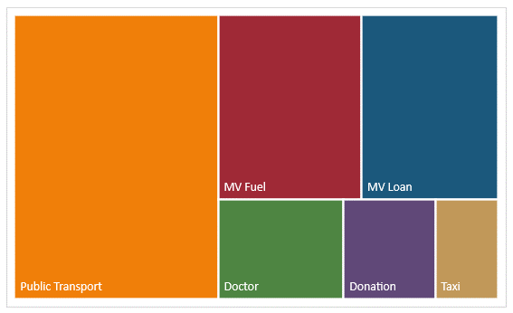
But with dynamic named ranges we can trick them into referencing the PivotTable as the source data.
4.1 Create Dynamic Named Ranges
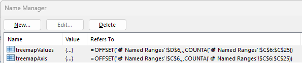
Use the OFFSET function to create a dynamic named range for both the series values and axis labels.
4.2 Define Names
Convert the OFFSET formulas to defined names, such as `treemapAxis` and `treemapValues`.
4.3 Edit Chart Source
Replace cell references in the chart data
source with the dynamic named ranges.
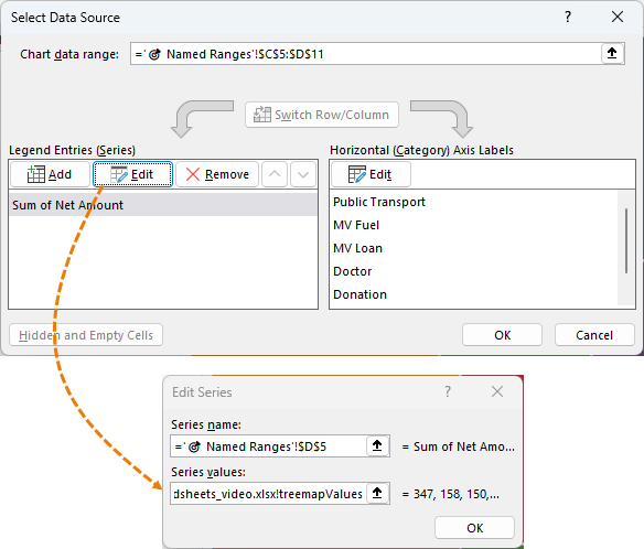
This allows your charts to update dynamically when data changes.
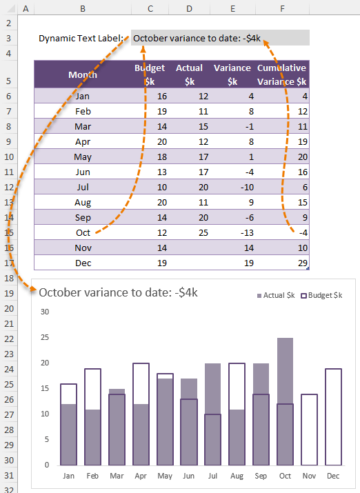
5. Dynamic Labels
Creating dynamic text labels that update automatically can save a lot of manual work. For example, the title of this chart automatically updates as new data is added to the Actual column of the table:
5.1 Extract Label Data
Use
INDEX and MATCH functions to return the month and cumulative variance for the latest data:
Latest month:
=INDEX(Table1[Month], MATCH(1E+10,Table1[Actual
$k],1))
Latest cumulative variance:
= INDEX(Table1[Cumulative Variance $k], MATCH(1E+10,Table1[Actual $k],1))
5.2 Format and Combine Text
Use the TEXT function to format the date and number values appropriately, then combine them into a single formula.
=TEXT(
INDEX(Table1[Month]
MATCH(1E+10,Table1[Actual $k],1)), "mmmm")
&" variance to date: "&
TEXT( INDEX(Table1[Cumulative Variance $k],
MATCH(1E+10,Table1[Actual $k],1)),
"$#,###0k;-$#,##0k")
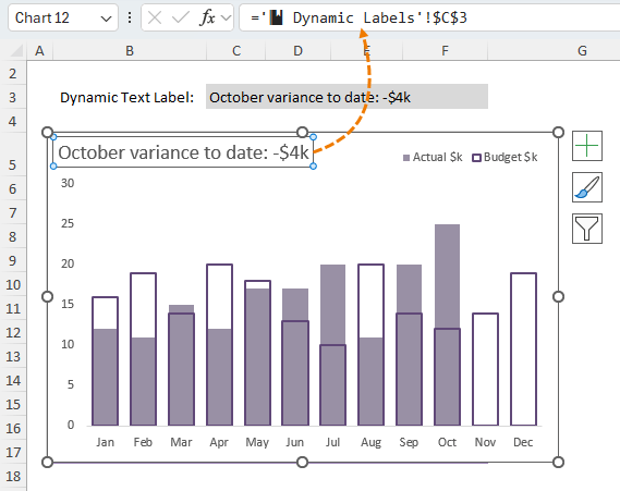
5.3 Link Label to Chart
Link the cell containing the dynamic label to the chart title, so it updates automatically with new data.
Next Steps
With these tricks, your Excel spreadsheets will update themselves, freeing you from endless manual
updates and giving you more time to focus on what really matters.
Unlock your potential with our Excel and Power BI courses! Join thousands who are mastering essential skills,
getting noticed, and earning promotions with our expert tips and tricks.