Inefficient References
First, let's look at a common example of an inefficient formula: below in columns A and B we have some employee data, and in columns E and F we’ve set up a COUNTIF formula (we can see the actual formula from column F in column G):
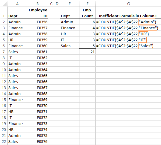
While this formula is technically correct, it's inefficient to write.
Let me explain; the ‘criteria’ argument (in the orange boxes in the image above), has been entered as text and this means each formula in column F had to be modified for each department. That's way too much work.
A more efficient way to write the formula
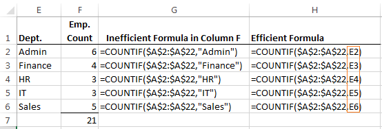
is to reference a cell for the criteria argument as you can see in the example in column H below (especially since it’s right there in column E):
Formulas written this way are:
- Quick: with the efficient formula (as shown in column H above) you enter your formula in cell F2 and then copy it down the column and your job is done.
- Easy to Update: if you need to change the Dept. names in column E, your formula will automatically pick up the new name without the need to also edit the formula.
- Intuitive: where there are formulas in contiguous cells experienced Excel users will expect that the formula can be copied and pasted to all adjacent cells.
So if someone inherits your file and they edit the formula, they will do so in the top left cell in the range of formulas and then copy and paste it to the remaining cells in the table. However, this could result in errors if, for example, they don't notice that your formulae 15 rows down and 3 columns to the right are subtly different because you hard keyed some criteria!
Absolute vs Relative References
Another hallmark of an efficient formula is its adept use of absolute and relative references. Those $ symbols within a formula denote whether a reference is fixed or dynamic.
Think of an absolute reference as fixing a cell's location, ensuring it remains constant, regardless of where the formula is copied to. On the other hand, a relative reference is adaptable, changing relative to the
number and direction of cells it has moved.
When copying a formula, any row or column references marked by a $ symbol stay the same, signifying they're absolute. In contrast, references lacking the $ symbol automatically adjust relative to their new location.
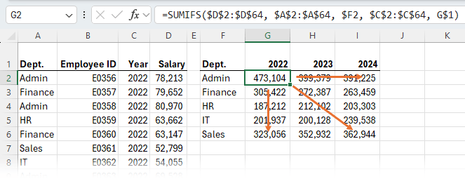
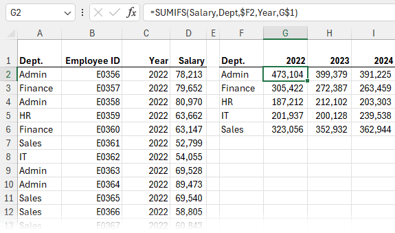
Below is an example where absolute and relative references enable me to copy and paste one formula to
many cells, earning its weight in gold; the SUMIFS formula in cell G2 (as seen in the formula bar below) can be written once and copied to the remaining 14 cells in the summary table:
As opposed to this inefficiently written version of the formula in cell G2:
=SUMIFS($D$2:$D$64,$A$2:$A$64,"Admin",$C$2:$C$64,2022)
Notice the difference between the efficient
formula and the inefficient one. The inefficient formula would require you to enter 15 different formulas, whereas the efficient formula is entered once and then copied and pasted to the remaining cells in the table.
Notice how some cell references have the column and row references absolute like this: $D$2
Some just
have the column reference absolute: $F2
And others just have the row reference absolute: G$1
I won't go into detail on this here, instead you can read my tutorial on absolute and relative
references.
If you haven’t mastered absolute and relative references yet I recommend you put them at the top of your ‘Excel To-Learn list’.
Named Ranges
The above tips will help you leverage Excel and absolute/relative references
to do a lot of the work for you, and it's a great start but, those cell references make the formula tricky to read and write.
Let's do better by using Named Ranges instead of cell references.
For example our previous SUMIFS formula can also be written like this (see formula bar below):
Now, isn’t that easier to read? It's also quicker to write since you can type the name of the range into the formula or press F3 to bring up the list of names to choose from.
Named ranges in their simplest form allow us to give a range of cells a name which can then be used in place of the actual cell references.
For example we can give the following ranges used in our SUMIFS formula names:
- $D$2:$D$64 name is ‘Salary’,
- $A$2:$A$64 name is ‘Dept’
- $C$2:$C$64 name is ‘Year’.
So now this formula:
=SUMIFS($D$2:$D$64,$A$2:$A$64,$F2,$C$2:$C$64,G$1)
Can be written like this:
=SUMIFS(Salary,Dept,$F2,Year,G$1)
Click here to see how to set up Named Ranges.
If you’ve mastered
Named Ranges then you might be interested in Dynamic Named Ranges. These are ranges that expand and contract automatically (dynamically) as your data expands and contracts, or based on criteria you stipulate.
You can create a dynamic
range using the OFFSET function or INDEX function however, if the thought of using those is a bit
scary then there is a very easy way to create dynamic ranges using Excel Tables.
Excel Tables
I’m going to be blunt here; if you aren’t familiar with Excel Tables then you are missing out.
These are one of the most useful features that came out way back in Excel 2007 and yet they are one of the most underused.
The following features of Excel Tables are going to revolutionise the way you write formulas:
- Structured References: This is the name given to the way you reference cells in an Excel Table. Structured references work in a similar way to Named Ranges however, since they’re part of the Excel Table features you don’t need to set them up manually.
- Dynamic Ranges: The Structured
References are dynamic; this means as you add new data to your Table the ranges automatically grow to incorporate that new data.
Structured References are a great alternative if the idea of having to get your head around complicated OFFSET or INDEX formulas to build your dynamic named ranges doesn't appeal.
Working with
Structured References
There are various ways to reference the components of the Table, and in the example below you can see these particular references are made up of the table name (Table1), and column label, which we can either type in or choose from a list.
This ability to choose from a list is one of the great features of Excel Tables. As you type in part of the
table/column name a list of names you can use becomes available (similar to named ranges), and you simply select the one you want.
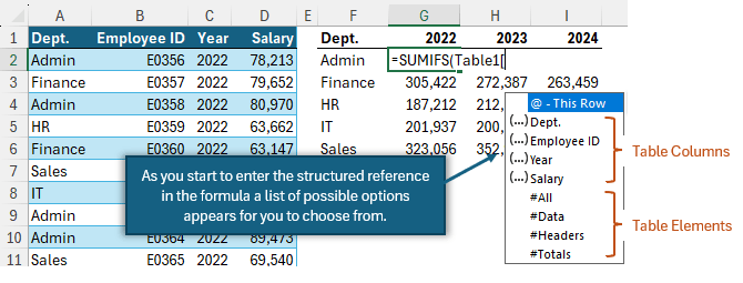
With structured references our formula in G2 becomes:
=SUMIFS(Table1[Salary],Table1[Dept.],$F2,Table1[Year],G$1)
The named ranges have been replaced with the table’s structured
references (e.g. Table1[Salary] etc.)
There are many more features that come with Excel Tables which I consider a bonus:
- Filter buttons automatically applied
- Banded row formatting
- Flexible Total Row formula using Subtotal
- Automatic Freeze Pane for column labels
- Streamline your work with my Excel Tables course.
Spilled Arrays
With the introduction of Dynamic Array formulas, we can now use the hash sign shortcut to quickly reference spilled arrays.
For example, here I've used the UNIQUE Function to extract a list of the departments from column A. I can then reference the list of departments in my COUNTIF formula using the shortcut E2#. This returns a spilled array of the employee counts:
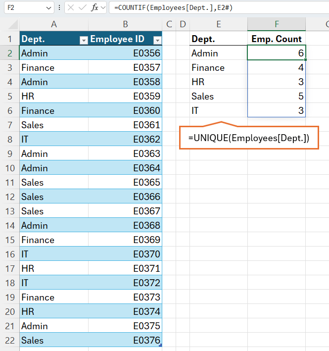
This is quicker to reference and write, plus I don't have to copy it down the column because it spills the results for me.
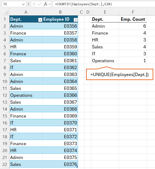
And if a new department gets added, the formulas automatically pick it up, as you can see in the example below for the new department,
'Operations':
We can also reference spilled arrays in data validation
lists and more. Check out this comprehensive tutorial on the spilled array operator for more tricks.
The Upshot
The bottom line is your formulas should and can be quick to write,
interpret and update.
You should be aiming to write one formula for the top left cell in your table, or first cell in your column of formulas and then copy it to everywhere it needs to go. Any alterations to ranges or criteria etc. should dynamically update based on the destination of where you paste the formula.
Tools we can use to help:
- Absolute and relative references
- Named ranges
- Excel Tables
- Spilled Arrays
- Troubleshooting Excel Formulas
Next Steps
Now that you have one less Excel problem and more free time to dedicate to other important tasks. Want to save even more time? There’s a common Excel mistake most overlook, and I've explained it in this tutorial along with a solution. Check it out to avoid falling into this trap and elevate your Excel expertise even further. See you there!