Function vs Formula
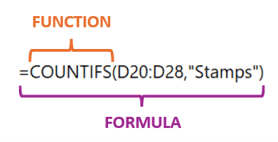
Before we start, I want to clarify the difference between a function and a formula because these terms are often incorrectly used interchangeably.
Excel formulas are the instructions you write to perform calculations or manipulate data.
They start with an "=" sign and can combine numbers, cell references, and operations like addition or subtraction, as well as functions.
Functions, on the other hand, are built-in shortcuts for common calculations - think of them as recipes to which you just add ingredients.
UNIQUE Function
With the UNIQUE function we can instantly clean our data sets, removing duplicates or extracting a list of distinct items for use in other Excel tools like data validation.
It's available in Excel for Microsoft 365 and Excel 2021 onward.
UNIQUE function syntax:
UNIQUE(array, [by_col], [occurs_once])
array is the range or array you want the unique values returned from.
by_col is an optional logical value (TRUE/FALSE) and allows you to compare values by row (FALSE), or by column (TRUE).
occurs_once is also an optional logical value (TRUE/FALSE) and allows you to find the truly unique values, i.e. the values that only occur once (TRUE), or
all distinct values (FALSE). If you omit this argument, it will default to FALSE and return a distinct list.
UNIQUE Function Example
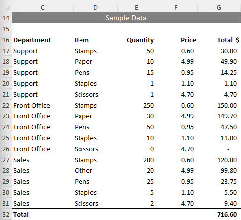
Let's say I want to extract a distinct list of the items in column D from the table below:
It's easy with the UNIQUE function like so:
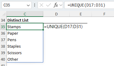
The UNIQUE function spills the results to the cells below.
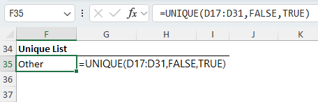
Alternatively, I can return items
that are unique, that is, there is only one instance of them by specifying TRUE in the 'occurs_once' argument:
You can also use the UNIQUE function to reference multiple columns and compare whole rows, which is handy for removing duplicates from your data.
SORT Function
With the SORT function we can organize data in ascending or descending order, automatically transforming an unmanageable list into a neatly ordered dataset in no time.
SORT function syntax:
SORT(array, [sort_index], [sort_order], [by_col])
array is the range or array containing the values you want sorted.
sort_index is optional and indicates the row or column to sort by. When omitted it will default to sort by the first row
or column in the array.
sort_order is optional. It's a number; 1 for ascending and -1 for descending. If omitted, it will sort in ascending order.
by_col is an optional logical value (TRUE/FALSE) indicating the desired sort direction; FALSE to sort by row
(default), TRUE to sort by column. Most of the time you'll want to sort by row.
SORT Function Example
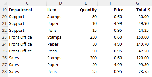
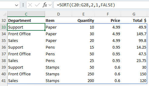
For example, let's say we want to sort this table based on the items in ascending order:
When writing the formula, the array is the whole table. The index is the column I want to sort by, in this case the second column. The sort order is 1 for ascending order
and the sort direction is FALSE to sort by row:
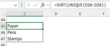
SORT
is super handy for using with other functions, for example, we could use it with UNIQUE to sort a list of items we extract:
TEXTJOIN Function
Better than CONCAT, TEXTJOIN combines text from multiple cells or ranges. Plus, it can ignore blanks and include a delimiter, making data concatenation seamless.
TEXTJOIN Function Syntax:
TEXTJOIN(delimiter, ignore_empty, text1, [text2],...)
delimiter - this is what you want each text string separated with. It can be another text string, a reference to a cell
or an empty space, all surrounded by double quotes. Note: if a number is provided it will be treated as text.
ignore_empty- this is either TRUE (you want it to ignore empty cells in your range), or FALSE, or their numeric equivalents of 1 and 0.
text1- this is
the text you want to join, it can be a text string, a range of cells, or an array of strings.
text2...- You can continue adding text to join, up to a maximum of 252 including Text1. Note: the maximum length of the resultant text string is 32767 characters.
TEXTJOIN Function
Example
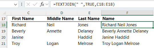
Here I have a table of names separated into first, middle and last names, and in column F I've used TEXTJOIN to join them together into one column with a space delimiter:
Check out the video above for another cool way to use TEXTJOIN to create a dynamic title for use with Slicers.
FILTER Function
The FILTER function is my favourite! It allows you to filter data based on criteria you specify. The output can be displayed in the worksheet or fed into another function. It's immensely versatile.
FILTER Function
Syntax:
FILTER(array, include, [if_empty])
array is the range or array containing the values you want filtered.
include is the logical test that returns a Boolean array (TRUE/FALSE) the same height or width as the array.
if_empty is an optional value to return if the included array are empty i.e. if the filter results in no records.
FILTER Function Example
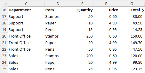
Let's say I want to extract the Sales department's data from this table:
The first argument is the array I want to filter, which is my data table.
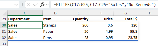
Next, I specify what rows I want to include with a logical test. In this case I want to filter the rows where the Department = 'Sales'.
The last argument allows me to specify a value to return if there are no results based on my
criteria, for example, I could return the text 'No Records'.
And just like that, I've filtered my list:
You can also do things like link it to a data validation list and make it dynamic. Plus, you can include multiple filter criteria, return specific columns, and rearrange the order of columns and more which I cover in my comprehensive
FILTER function tutorial.
VSTACK Function
The VSTACK function vertically stacks arrays or ranges or data, which is ideal for consolidating
data without the need for complex formulas or Power Query.
Syntax:
VSTACK(array1,[array2],...)
array The arrays (cell
ranges) you want to append.
VSTACK Function Example
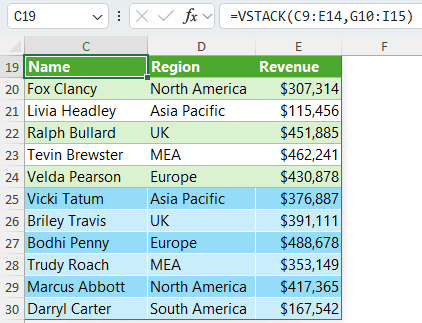
Here I have two tables, they could be on separate sheets and I want to consolidate them into one table.
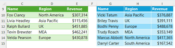
All I need to do is select the first range, and I'll include the headers. And then include the second range. Job done!
VSTACK also has a sibling function called HSTACK for horizontal stacking and I cover that and more cool ways to use VSTACK in this tutorial.
Deep Dive
We have only scratched the surface of what Excel functions can do. My Advanced Excel Formulas course is here to transform you into an Excel wizard, offering in-depth insights into complex formulas and data analysis techniques. Elevate your skills, streamline your workflow, and stand out as the go-to Excel expert.

XLOOKUP Function
The XLOOKUP function is the new improved VLOOKUP. It's the Swiss Army knife of lookups, offering a versatile way to find and retrieve information across a table or range without the shortfalls of VLOOKUP or the complexities of INDEX & MATCH.
Syntax:
XLOOKUP( lookup_value, lookup_array, return_array, [if_not_found], [match_mode], [search_mode])
lookup_value The value you want to find, or cell containing the item you want to find
lookup_array The cell range or array you want to search return_array The cell range or array containing the value you want returned
[if_not_found] Optional - the text you want returned in the event a match isn't found. If omitted an error will be returned.
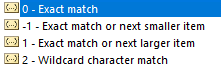
[match_mode] Optional - Defaults to 0 for exact match
[search_mode] Optional - Defaults to 1 searching first to last
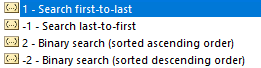
Options 2 and -2 require the lookup_array to be sorted in ascending or descending order respectively.*
*Binary search does not result in faster calculations now that Microsoft have optimised the lookup algorithms.
XLOOKUP Function Example
Let's say I want to lookup the product 'Caps' in the table below and return the sales. It's super easy with XLOOKUP:
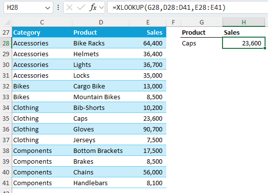
Unlike VLOOKUP, XLOOKUP defaults to return an exact match, so there's less risk of formula errors, and I think you'll agree, it's easier to write.
Of course, there's more arguments that allow you to handle errors and return a value if the match isn't found, so check out this comprehensive XLOOKUP tutorial.
SEQUENCE Function
The SEQUENCE
function generates a list of sequential numbers, perfect for creating custom data series or time sequences with minimal effort. You might be thinking you'll never need this function, but it's more versatile that it first appears so stay tuned.
Syntax:
SEQUENCE(rows, [columns], [start], [step])
rows Here you specify the number of rows to be returned.
columns is optional and specifies the
number of columns to be returned. If omitted it will return 1 column.
start is optional and specifies the first number in the sequence. If omitted it will start at 1.
step is optional and specifies the increment for each
subsequent value in the array. If omitted it will increment by 1.
SEQUENCE Function Example
Let's say you're using Excel to create a list of items and you want to number them. It's super easy with sequence.
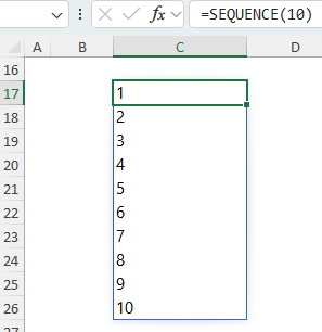
And if I insert or delete a row, the numbering doesn't get messed up.
But like most functions,
when you team it up with other functions you can make magic happen. Let's say I want a list of month end dates.
I can use the EOMONTH function to return the month end dates, and in the month argument I'll use SEQUENCE to return 12 values starting at zero:
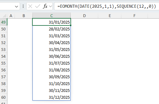
If you wanted 2 years' worth of dates, you could simply change 12 to 24.
Next time you
need a list of numbers or dates, consider using SEQUENCE to speed up the process.
TEXTSPLIT Function
The TEXTSPLIT function divides text into separate columns based on a
delimiter, which is way easier than the old LEFT, MID, RIGHT function combination we had to wrangle.
Syntax:
TEXTSPLIT(text, col_delimiter, [row_delimiter], [ignore_empty],
[match_mode], [pad_with])
input_text The text you want to split. Required.
col_delimiter One or more characters that specify where to spill the text across columns. Optional.
row_delimiter One or more characters that specify where to spill the text down rows. Optional.
ignore_empty Specify TRUE to create an empty cell when two delimiters are consecutive. Defaults to FALSE, which means don't create an empty cell. Optional.
match_mode
Searches the text for a delimiter match. By default, a case-sensitive match is done.
pad_with Text entered in place of blank results.
TEXTSPLIT Function Example
Here I have a list of names and I want to split them into separate columns for First, Middle and Last name.
All I need to do is reference the cell containing the name and then specify the delimiter:
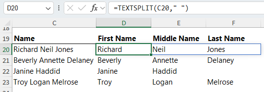
Note that TEXTSPLIT wasn't able to correctly parse Janine Haddid because there's no middle name, so you do have to be careful that your data is consistent.
There are some other arguments we can use with TEXTSPLIT and it has some sibling functions TEXTBEFORE and TEXTAFTER that are also super useful, so check out this comprehensive tutorial TEXTSPLIT, TEXTBEFORE and TEXTAFTER.
IFS Function
Easier than nested IF formulas, the new IFS function is a streamlined alternative, allowing multiple conditions to be evaluated in a single, elegant formula.
Syntax:
IFS(logical_test1, value_if_true1, logical_test2, value_if_true2, logical_test3, value_if_true3, ... )
logical_testN is the logical test that returns a Boolean (TRUE/FALSE
value_if_trueN is the result
to be returned if logical_test evaluates to TRUE. Can be empty.
IFS Function Example
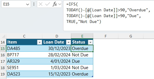
Here I have a list of items that are out on loan, and I want to check their status where Loan items > 90 days old are overdue, items = 90 days old are due and items < 90 days old are not due.
This last argument is not very intuitive, so let's step through the formula.
IFS works in pairs of arguments, the first is the logical test, if it's true, it returns the corresponding value if true. If it's false, it moves onto the next logical test and so on.
In this case, if the first two logical tests are false, so it moves onto the third logical test and I could put TODAY() - loan date < 90, but if the first two logical tests are FALSE, then this must be TRUE, so I can
simply skip this last logical test and put TRUE here.
Next time you need to write a nested IF formula, consider using IFS instead so you don't have to deal with the nightmare of multiple sets of closing parentheses.
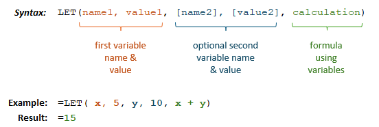
LET Function
With the LET Function you can say goodbye to repeating complex calculations and make formulas much easier to write and read when you come back to them months down the track.
LET Function Example
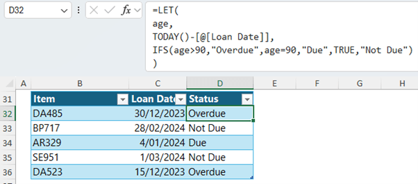
In the previous example we used a formula to classify loan items and that formula used the same calculation multiple times. A more efficient way to write this formula is with LET.
With LET I can
declare variables and intermediate calculations inside the formula. Using the previous formula I can declare the TODAY()-[@[Loan Date]] as a variable called 'age'.
My formula then becomes:
=LET(
age,
TODAY()-[@[Loan Date]],
IFS(age>90,"Overdue",age=90,"Due",TRUE,"Not Due")
)
Looking at the formula now, it's not only more efficient for Excel to calculate because the age is only being calculated once, but it's also easier to read.
Next time you find yourself repeating calculations inside a formula, or you're writing a long complex formula, consider using LET for efficiency and clarity.
Next Steps
Keeping up to date with
new functions like these is just one piece of the Excel productivity puzzle.
Whether it's creating invoices, project plans, or regular reports the monotony of performing these repetitive tasks each time from scratch can be mind-numbing and time-consuming.
That's why I recommend you check out 10 Excel tools designed to save you time on everyday tasks next. I'll see you there.