Excel Checkboxes in Cells
Checkboxes are a great tool for making selections or indicating choices.
Before these new in-cell checkboxes were released, Excel had form control checkboxes. However, these were quite tedious to work with and had their limitations.
To simplify using checkboxes, Excel has now made it possible to insert checkboxes in cells. This creates a more intuitive and integrated spreadsheet experience.
Practical Applications
Incell
checkboxes have diverse applications, such as simple task lists, enabling and disabling data displayed in charts, and turning on and off conditional formatting to name a few.
Let’s look at some of these applications with some examples.
Task Lists
Suppose you are going on a trip and packing seems too daunting a task. Use in-cell checkboxes to make it
much simpler for you.
List down everything you need to pack in an Excel sheet. Then use the next two columns to categorize items under “Do I have these?” and “Have I packed these?” categories.
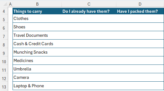
Now, you have a nice-looking matrix and are ready to insert checkboxes.
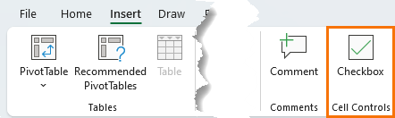
Select the cells to insert checkboxes > Go to Insert Tab > Select Checkbox under Cell Controls
You can even insert a 4th column for Status.
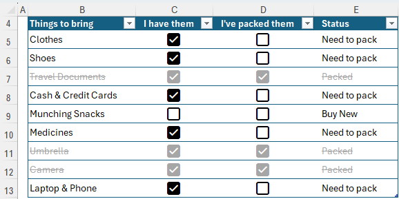
These checkboxes have TRUE/FALSE values when checked and unchecked, respectively.
You
can create a nested IF formula that tells you what you need to do – i.e. do you need to buy something, pack it, or you have already packed it.
=IF(D5,"Packed",IF(C5,"Need to pack", "Buy
New"))
Tip: because the checkbox returns TRUE and FALSE as their status, we don’t need to perform further logical tests, we can simply reference the cell status.
The status column tells you what you need to pack and buy.
This way, you can generate a task list and a buying list at the same time.
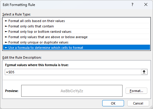
For a finishing touch, add conditional formatting to format the font in grey and a strikethrough.
Home tab > Conditional Formatting > New Rule > Use a formula to determine which cells to format:
Project Management
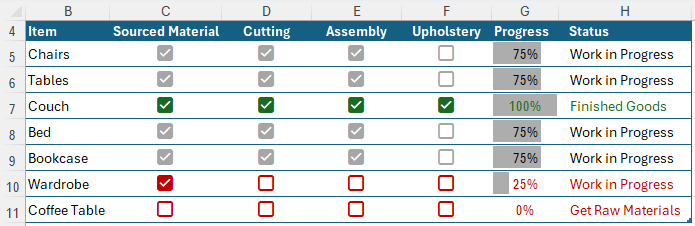
Similarly, you can use these checkboxes to track the progress of a multi-step production process, such as furniture manufacturing.
You can list down several items and the processes they undergo, and track production progress, by simply combining these in-cell checkboxes using data bars and conditional formatting.
To do this, you first need to calculate the progress percentage
using the below formula:
=IFERROR(COUNTIF(C3:F3,TRUE)/COUNTA(C3:F3),"")
Here COUNTIF adds up the check-marked processes and divides it by the total number of processes, calculated using COUNTA.
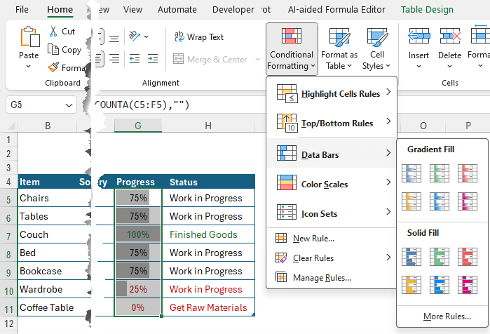
Next, insert the
Conditional Formatting data bars.
Select cells G5:G11> Home Tab > Conditional Formatting > Data Bars > Pick any one from Solid or Gradient Fill Data Bars.
Here, I have also added the rules that make the font color of the cells change based on progress rate -
Green when 100% and Red when < 30%.
You can even add progress-based dynamic remarks and then use those remarks to filter the rows.
For example, here we can categorize the progress into the 3 inventory heads – Raw Material, Work in Progress, and Finished Goods, by using a simple IF and SWITCH function combination:
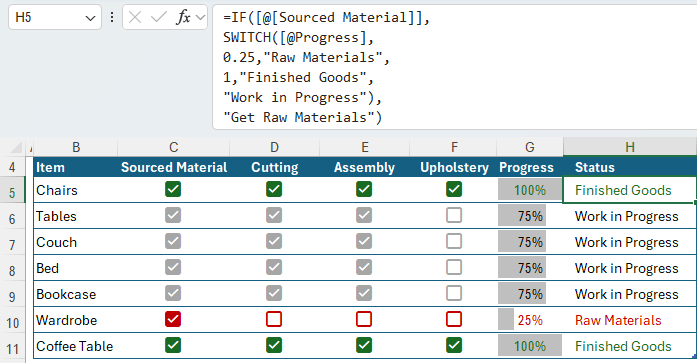
=IF([@[Sourced Material]], SWITCH([@Progress], 0.25,"Raw Materials", 1,"Finished Goods", "Work in Progress"),"Get Raw Materials")
The IF function assesses whether the “Sourced Material” checkbox is checked or not.
If it is checked, it implies that the manufacturer has the materials. Only after this, the SWITCH function comes into play.
SWITCH function categorizes the inventory into 3 statuses as follows:
Progress Rate | Status | Reason |
25% or 0.25 | Raw Materials | Only “Sourced Material” checkbox is checked |
100% or 1 | Finished Goods | All 4 checkboxes are checked |
Any other value in between | Work in Progress | Some tasks remain to be completed. |
However, if Sourced Material is FALSE, the SWITCH function is ignored, and the IF function returns its FALSE value, i.e. “Get Raw Materials”.
Dynamic Charts
For a more sophisticated use you can combine these checkboxes with charts to toggle which series to display.
They can come in very handy in data analysis and interactive dashboards.
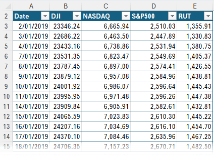
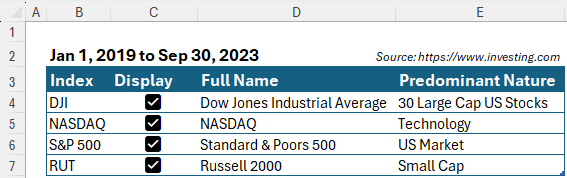
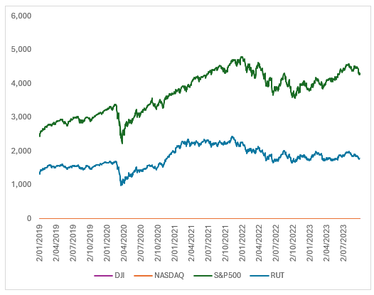
The chart displays historical data of 4 US stock market indices from Jan 1, 2019 to September 30, 2023.
To set it up:
- Create a new table with the names of the indices and the checkboxes.
- Create a new data table linked to the original one. However, this table will only display index prices if you have the corresponding checkbox
checked.
- Bring the dates in from the source table, copy and paste if you don’t expect it to change, or use a formula as shown below.
- Use XLOOKUP to find the corresponding price of the index on that particular date.
- Multiply the output with the checkbox cell of the corresponding
index.
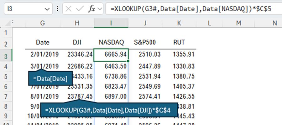
The formula in column H is:
=XLOOKUP(G3#,Data[Date],Data[DJI])*$C$4
You will need to adjust the multiplier to the corresponding check box for each index.
Now when you check the checkbox for an index, the new data table will show its prices, but when you uncheck it, the
prices will become 0.
Tip: if you prefer to hide the line altogether, use IF to return N/A like so:
=IF(C4, XLOOKUP(G3#,Data[Date],Data[DJI]), NA())
- Using this
new data table, insert a line chart which will also be dynamic, and only display the indices you checkmark.
This functionality is helpful when viewing multiple series in a single chart where those series are significantly different in scale.
For example, DJI and NASDAQ appear to have been more volatile over the
period than the S&P 500 and RUT, which appear relatively flat.
However, if you remove DJI and NASDAQ from the chart, you can see that they were also volatile, just on a smaller scale.
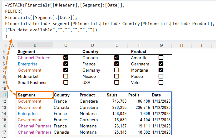
Filtered Lists
We can team incell checkboxes up with the FILTER function to enable users to select what data they want
returned in a table.
The source data table called ‘Financials’ has some
helper columns (H through J) to detect if the checkbox on the sheet called ‘ FILTER’ is selected for the data in the row:
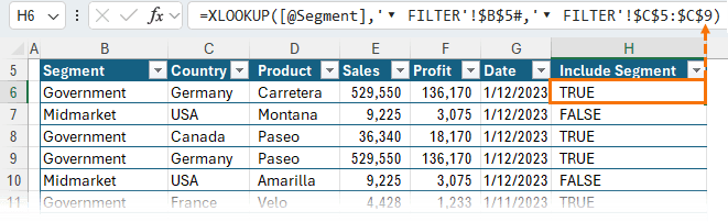
Then the VSTACK function brings the headers from the Financials source table and joins them to the top of the table returned by the FILTER function;
See the video above for step-by-step instructions or download the file above.
Key Features of the New
Checkboxes
The introduction of in-cell checkboxes brings several advantages:
Simple Insertion: Easily add checkboxes directly into cells from the `Insert` tab.
Enhanced Data Integrity: These checkboxes maintain
their position and alignment, even with changes to the spreadsheet layout because they are part of the cell.
Compatibility with Conditional Formatting: Leverage Excel's conditional formatting features in conjunction with checkboxes for dynamic data visualization.
Limitations
- You can trigger checking the
checkbox with a formula, but you can’t also manually check the box.
- Does not auto-fill down in tables
- Deleting a checkbox converts it into a ghosted state that can be brought back when you click on the cell. To remove it completely you must clear all formats via the Home tab.
- If you open
the Excel file in a version of Excel that doesn’t support the new checkboxes, the cells will simply display TRUE or FALSE.
- Checkboxes don’t display in data validation or PivotTables, however their TRUE and FALSE values do.
Additional Resources
If you don’t have the new in-cell checkboxes, try the original form control check boxes here.