Excel Dynamic Named Ranges with INDEX
Most people think of the OFFSET function for dynamic named ranges. Unfortunately, OFFSET is volatile, meaning it recalculates even if none of its arguments have changed, leading to more frequent updates and potential performance issues.
In general, it's a good practice to be mindful of the use of volatile functions, especially in large or complex Excel files, to ensure that they don't
inadvertently slow down your work.
I prefer to use the INDEX function for dynamic named ranges.
INDEX has two syntax options, and for dynamic named ranges we use this version:
Syntax: =INDEX(array, row_num, column_num)
array – the range of cells you want to return a range from.
row_num – the row(s) you want to return.
column_num – the column(s) you want to return.
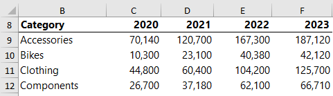
Applying it to this example data:
I like to write my dynamic named range formulas in a cell
in the worksheet as it’s easy to construct them using the mouse to select the ranges and I can test they work as expected before defining them as a name.
Return a Range with Flexible Last Row and Column
This type of dynamic named range is useful as the source for PivotTables, and lookup formulas where you want to look up an entire table.
I can use INDEX with the COUNTA function to determine the current size of the table and return the range.
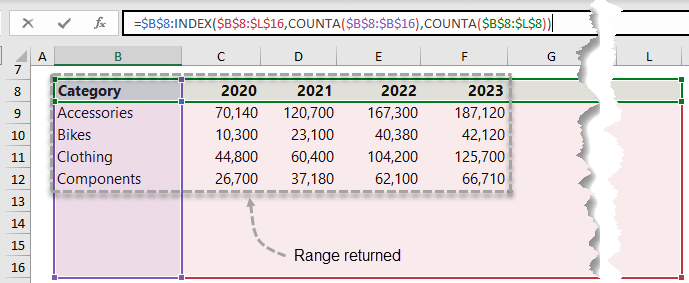
I’ve
allowed for growth to row 16 and column L, as shown in the image below with the grey dashed line indicating the range that will be returned by the formula:
Each argument explained:
=$B$8
The first cell in the range I want returned. In this case it will always be the top left cell. Tip: if you don’t need the header row in the range, start at cell B9 and adjust the row_num COUNTA formula to also start in row 9.
:
Colon range operator.
INDEX(
Use INDEX to find the last row and column in the table using COUNTA for the row and column arguments.
array
=$B$8:$L$16
Select cells that represent the maximum size table will potentially grow
to.
row_num
COUNTA($B$8:$B$16)
Counts the row labels in the first column to determine the current height of the table. The height of this range must match the height of the INDEX range and should not
contain any empty cells.
column_num
COUNTA($B$8:$L$8))
Counts the column labels in the first row to determine the current width of the table. The width of this range must match the width of the INDEX
range and should not contain any empty cells.
Note: when writing formulas for dynamic named ranges make sure the cell references are all absolute references.
Return a Range
for a Specific Row
Sometimes you only need one row returned. It could be based on a selection in a data validation list or another cell, for use in a chart, table or a formula.
For example, below I can choose a different category from the data validation list and the values are returned and displayed in the chart.
Note: Excel 2019 and earlier users will not be able to display the values being returned by the formula in the grid (cells C38:F38) as you do not have dynamic array functionality. However, you can
skip this step and simply define the formula as a name for use in charts etc.
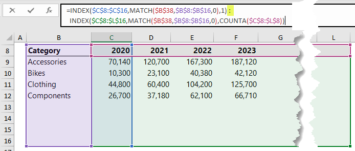
The formula for returning a range for a specific row uses INDEX and MATCH on both sides of the colon range operator:
Each argument explained:
=INDEX(
Use INDEX to find the first cell in the range you want returned.
array
$C$8:$C$16
The first cell I want returned is in the first value column of the table (column C) and I’ve allowed the data to grow to row 16.
row_num
MATCH($B$38,$B$8:$B$16,0),
MATCH is used to find the row the category selected in cell B38 is on, in the range B8:B16.
column_num
1)
Technically this argument can be skipped as only one column is selected in INDEX’s array argument, but I’ve entered 1 for completeness.
:
Colon range operator
INDEX(
Use INDEX to find the last cell in the range.
array
$C$8:$L$16
The range containing the last cell, allowing for growth in rows and columns.
row_num
MATCH($B$38,$B$8:$B$16,0)
MATCH is used to find the row the category selected in cell B38 is on, in the range B8:B16.
column_num
COUNTA($C$8:$L$8))
Counts the column labels in the first row to determine the current width of the table. The width of this range must match the width of the INDEX range and should not contain any empty cells.
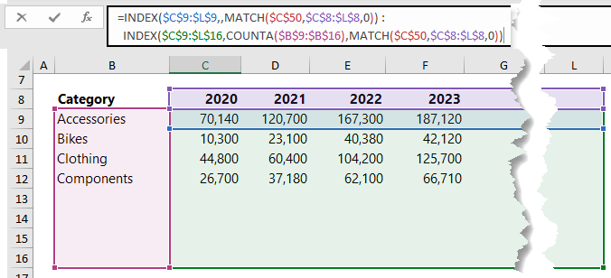
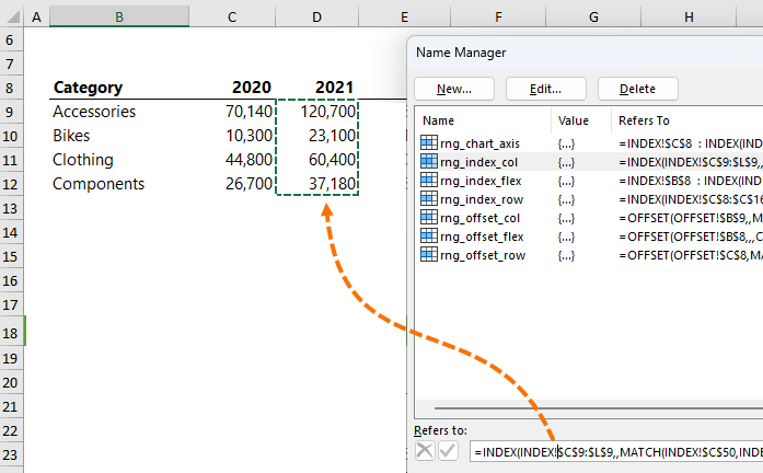
Return a Range for a Specific Column
Similarly, we can
use INDEX to return a specific column based on the selection made in the data validation list:
Note: Excel 2019 and earlier users will not be able to display the values being returned by the formula in the grid (cells C51:C54) as you do not have dynamic array functionality. However, you can skip this step and simply define the formula as a name.
The formula for returning a range for a specific column uses INDEX on both sides of the colon range operator:
Each argument explained:
=INDEX(
Use INDEX to find the first cell in the range.
array
$C$9:$L$9
The first cell I want returned could be in any column in the first row of the table and I’ve allowed the data to grow to column L.
row_num
This argument is skipped because there is only one row indexed,
therefore a row_num is not required.
column_num
MATCH($C$50,$C$8:$L$8,0))
MATCH is used to find the column for the year selected in cell C50 in the range C8:L8.
:
Colon range operator
INDEX(
Use INDEX to find the last cell in the range.
array
$C$9:$L$16
The range containing the last cell, allowing for growth in rows and columns.
row_num
COUNTA($B$9:$B$16)
Counts the row labels in the first column to
determine the current height of the table. The height of this range must match the height of the INDEX range and should not contain any empty cells.
column_num
MATCH($C$50,$C$8:$L$8,0))
MATCH is used to
find the column that the year selected in cell C50 is in the range C8:L8.
Defining Names
The power of these formulas comes when you define them with a name. That name can then be referenced multiple times in formulas, PivotTables, charts and more.
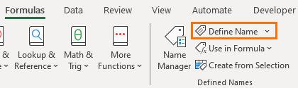
To define the
formula as a name, make sure all the references are absolute. Then copy the formula > Formulas tab > Define name:
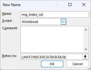
Name it and paste in the formula in the ‘Refers to’ field:
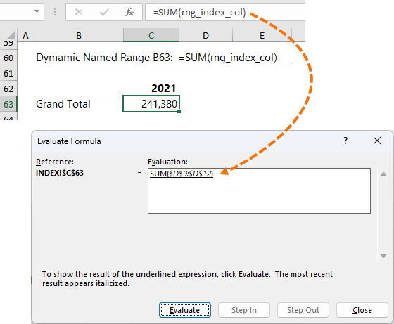
You can then reference the name anywhere you’d normally use a cell reference.
For example, in the image below I’ve summed the dynamic named range, and if I evaluate the formula, you can see that the defined name actually returns a reference to the range $C$10:$F$10
Dynamic Named Ranges with INDEX Key Points
Dynamic named ranges are incredibly flexible and with flexibility often comes complexity.
To summarize the key points:
- For dynamic ranges that you expect to grow,
INDEX a range larger than the current data size and use COUNTA in the row_num and column_num arguments.
- For dynamic ranges linked to drop down lists or other cells where the user can specify what they want returned, use MATCH in the row_num and column_num arguments.
- If the start and end of the range need to be flexible, use INDEX on both sides of the colon range operator.
- Ensure all cell references are absolute before creating the defined name. There are exceptions to
this which I cover in my Relative Named Range tutorial.
Excel Dynamic Named Ranges with OFFSET
The OFFSET function also returns a range that can be made dynamic with the use of the MATCH function and COUNTA.
However as mentioned above, it’s a volatile function and
therefore should be used sparingly.
Let’s recreate the same dynamic ranges using OFFSET to see how it compares.
Syntax: =OFFSET(reference ,rows, cols, [height], [width])
reference – the starting cell/range of cells
rows – the number of rows to move +/- from the starting cell to arrive at the first row in the range.
cols - the number of columns to move +/- from the starting cell to arrive at the first column in the range.
height – the number or rows high you want the range.
width – the number of columns wide you want the range.
Return a Range with Flexible Last Row and Column
This type of dynamic named range is useful as the source for PivotTables,
and lookup formulas where you want to look up an entire table.
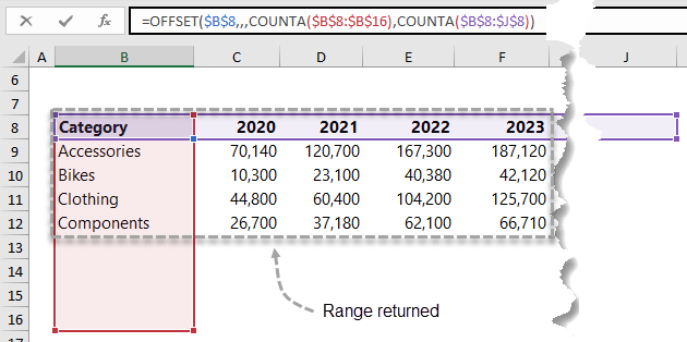
I can use OFFSET with COUNTA to determine the current size of the table and return the range.
I’ve allowed for growth to row 16 and column J, as shown in the image below with the grey dashed line indicating the range that will be returned by the formula:
Each argument explained:
=OFFSET(
reference
$B$8
The
first cell in the range will be the top left of the table.
rows
This argument is skipped because I don’t want to move down any rows from the reference cell before starting the range.
cols
This argument is skipped because I don’t want to move across any columns from the reference cell before starting the range.
height
COUNTA($B$8:$B$16)
Counts the row labels in the first column to determine the
current height of the table. This column should not contain any empty cells.
width
COUNTA($B$8:$J$8))
Counts the column labels in the first row to determine the current width of the table. This row should
not contain any empty cells.
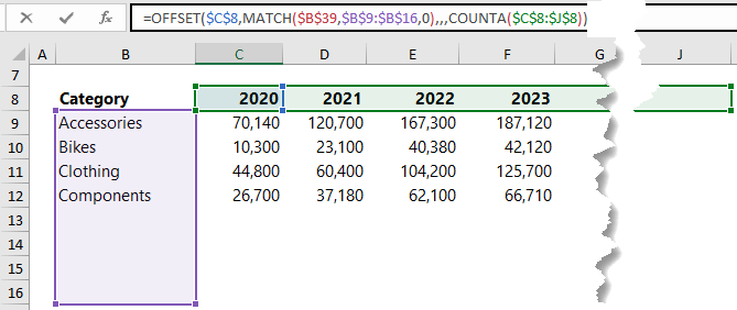
Return a Range for a Specific Row
Returning a specific row that’s based on a selection in a data validation list or another cell, for use in a chart, table or a formula is also doable with OFFSET.
The OFFSET formula also uses MATCH to locate the row for the category selected in cell B39 and COUNTA to determine the current width of the table:
Each argument explained:
=OFFSET(
reference
$C$8
The first cell in the range will be the first Year column label. Notice the reference starts in the header
row, because MATCH will return a value between 1 and 8, so at a minimum the starting cell will be 1 row below the reference cell.
rows
MATCH($B$39,$B$9:$B$16,0)
MATCH is used to find the row the
category selected in cell B39 is on in the range B9:B16. The lookup range allows for growth in the table to row 16.
cols
This argument is skipped because I don’t want to move across any columns from the reference cell
before starting the range.
height
This argument can be skipped because by default it will return 1 row.
width
COUNTA($C$8:$J$8))
Counts the column labels in the first row to determine the current width of the table. This row should not contain any empty cells.
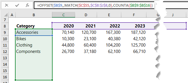
Return a Range for a Specific Column
Similarly, we can use OFFSET to return a specific column based on the selection made in the data validation
list:
Again, the OFFSET formula uses MATCH to find the relevant column and COUNTA to determine the height of the range.
Each argument explained:
=OFFSET(
reference
$B$9
The first cell in the range will be determined based on the year selected in the data validation list. Notice the reference starts in the row labels column because MATCH will return a value between 1 and 8, so at a minimum the starting cell will be 1 column to the right of the reference cell.
Rows
This argument is skipped because I don’t want to move down any rows from the reference cell before starting the range.
cols
MATCH($C$55,$C$8:$J$8,0)
MATCH is used to find the column the year selected in cell C55 is in, in the range C8:J8. The lookup range allows for growth in the table to column J.
height
COUNTA($B$9:$B$16))
Counts the row labels in the first column to determine the current height of the table. This column should not contain any empty cells.
width
This argument can be skipped because by default it will
return 1 column.
Using Dynamic Named Ranges in Charts
One of the best uses for dynamic named ranges is as the source for charts, enabling them to automatically update as your data grows or selections are made.
However, there are a few tricks to getting them to work with charts.
- You need a separate name for the axis labels and each series’
values.
- You need to prefix the name with the sheet name followed by an exclamation mark:
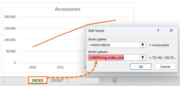
Note: after clicking ‘ok’ in the dialog box above, Excel will replace the sheet name with the
file name.
Troubleshooting Errors
The 3 most common causes of errors with dynamic named ranges are:
- Erroneous data entered in the cells being counted for the height or width.
If you inadvertently enter some data below or to the right of your table inside the area being counted, you will end up with a range larger than it
should be. - Blanks in the cells being counted for the height or width. The column you choose to count to determine the height of the range must not have any empty cells, otherwise the range will be smaller than it should be.
- Forgetting to absolute the cell references in the formula.
The easiest way to check the range being returned by a dynamic named range is to edit the range via the Name Manger (Formulas tab) and click in the Refers to field for the name you want to check.
Excel will put marching ants around the range being returned by the formula:
Relative Dynamic Named Ranges
So far, we’ve looked at dynamic named ranges that when referenced from anywhere in the workbook always return the same range. We achieve this by setting all references in the formulas as absolute.
However, we can also write relative named ranges
that return a range relative to the cell in which you refer to it from and they’re particularly handy.
For more see my Relative Named Ranges tutorial.
Alternatives to Dynamic Named Ranges
Dynamic named
ranges are a lot of work. It’s far easier to store your data in an Excel Table and use the built in Structured References that work like a dynamic named range by growing with your data.
Watch my video on Tables to learn more.