The Old, Slow Way
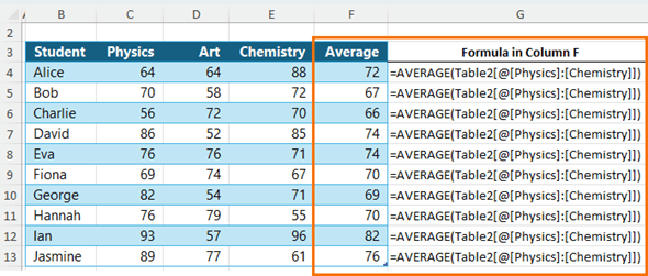
Before BYCOL and BYROW the only way we could automatically have an aggregation type of formula (SUM, AVERAGE, etc.) automatically fill down a column was to use an Excel Table.
In the image below, you can see the formula in column F is the same in each cell because it uses Table Structured References to refer to each row:
But what if you don’t want to or can’t use an Excel Table?
The next best option was to copy the formula down the column, but if we added more rows, we’d have to manually copy it down again.
The New Fast Way with BYROW Function
Now with the BYROW function, we can write one formula that automatically spills down a column.
It sounds counter intuitive because it’s called BYROW, but returns a column of values.
BYROW applies a function using LAMBDA to each row in an array and returns an array of equal height.
BYROW Function Syntax
BYROW( array, LAMBDA( arrayName, formula))
- array - the range of cells you want to pass to the LAMBDA formula one by one.
- arrayName – the name you give to the array in the first argument.
- formula – the formula you want to apply to each row in the
array.
BYROW Function Example 1
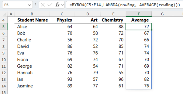
We can write one formula in cell F5 that calculates the average of each row and spills the results to the remaining rows like so:
The easiest way to think about BYROW is simply, any formula that you want to apply to one row, can automatically be applied to multiple
rows with BYROW.
=BYROW(C5:E14, LAMBDA(rowRng, AVERAGE(rowRng) ) )
In English it reads, pass each row in the range C5:E14 to LAMBDA to find the average for that row.
Step by step the formula can be
explained as follows:
- C5:E14: is the range of cells that the function will be applied to, one row at a time.
- LAMBDA allows you to define custom, reusable functions in Excel. It's like creating a mini-function on-the-fly without having to define a new named function in Excel
- roWRng: is the name given to the rows in cells C5:E14. Note: this name does not need to be defined in the name
manager, it is simply defined inside of LAMBDA. Whenever the LAMBDA function is called, it will operate on this row range.
- AVERAGE(roWRng): This is the reusable function. It calculates the average of the values in ‘rowRng’, which represents a single row from the range ‘C5:E14’.
BYROW Dynamic Ranges
We know that BYROW returns a spilled array of values
the same height as the array.
However, if we want to allow for more rows in the table to be added later without having to update the formula, we can reference more rows in the first argument with the TAKE function and
discard any empty rows before passing them to LAMBDA.
BYROW Function Example 2
Here I want to allow for more students to be added up to row 20 and automatically have the AVERAGE calculation in column F spill down to any new rows.
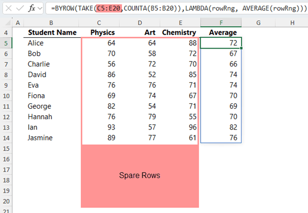
In the animated image below, you can see the AVERAGE calculation in column F automatically update to
include a new student on row 15.
BYCOL
Function
Like BYROW, the easiest way to think about BYCOL is any formula that you want to apply to one column, can automatically be applied to multiple columns with BYCOL.
The BYCOL function applies a function using LAMBDA to each column in an array and returns an array of equal width, spilling across a row.
BYCOL Function Syntax
BYCOL( array, LAMBDA( arrayName, formula))
- array - the range of cells you want to pass to the LAMBDA formula one by one.
- arrayName – the
name you give to the array in the first argument.
- formula – the formula you want to apply to each column in the array.
BYCOL Function Example 1
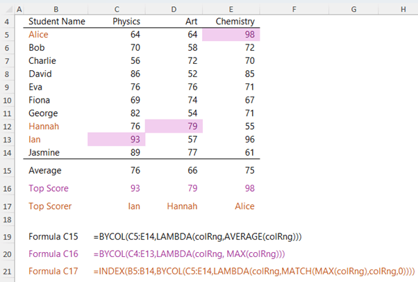
Let’s say we want to find the average scores for each subject.
The old way would be to write the formula in the first cell (C15) and then copy it
across the columns.
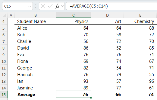
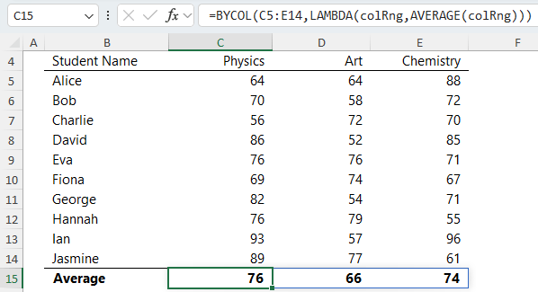
However, now with BYCOL, we can write it once in cell C15 and the results spill to the remaining columns.
BYCOL Function Example 2
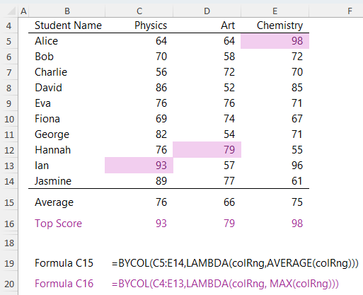
Let’s say we want to identify which student got the top score in each subject.
In row 16 we can easily identify the top score using MAX
In row 17 we can use INDEX and MATCH to return the student with the MAX score.
This formula can be explained as follows:
=INDEX(B5:B14, BYCOL(C5:E14, LAMBDA(colRng, MATCH(MAX(colRng), colRng, 0))))
In essence, the formula performs the following steps:
- For each column in the range C5:E14, use MATCH to find the row number where the maximum value of that column is located.
- Then uses that row number in INDEX to retrieve the corresponding
value from the range B5:B14.
Step by step the formula can be explained as follows
- INDEX returns the name from the range B5:B14 based on a row number that will be determined by the rest of the formula.
- BYCOL passes each column in the range C5:E14, to the LAMBDA.
- colRng is the name used by LAMBDA when referring to the columns in
the range C5:E14
- MATCH(MAX(colRng), colRng, 0): is the body of the LAMBDA function. Here's what it does:
- MAX(colRng): Finds the maximum value in the column range colRng one column at a time.
- MATCH(..., colRng, 0): Searches for the maximum value (found in the previous step) within the column range colRng and returns its relative position. The third
argument, `0`, specifies that we want an exact match.
BYCOL & BYROW Important notes
- If you’re familiar with LAMBDA, then it’s important to note that you do not need to define a name for the LAMBDA used by BYROW, although you can if you want.
- BYROW can evaluate a LAMBDA written inside it, without having to input the arguments inside parentheses at the end. e.g. this is not required:
=BYROW(C5:F14,LAMBDA(x,SUM(x))((C5:F14)))
- LAMBDA takes more than one name argument, but with the BYCOL function it can only take one name argument.
Related Lessons
Excel LAMBDA Function